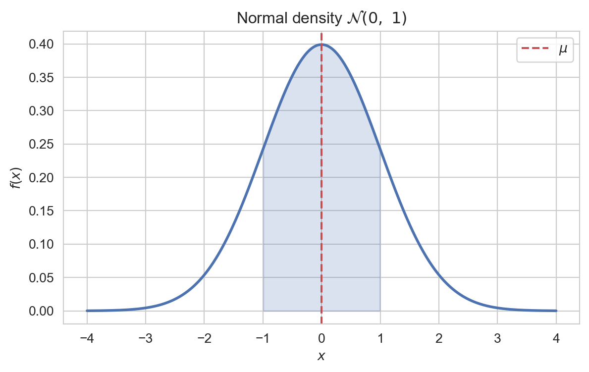
Normal Distribution – John Robin Inston

1 Introduction

The normal distribution (or Gaussian distribution) is a continuous probability distribution that is symmetric about its mean, with the familiar bell-shaped density. It arises throughout probability and statistics as the limiting distribution of normalised sums of independent random variables, via the Central Limit Theorem.

A random variable \(X\) follows a normal distribution with mean \(\mu \in \mathbb{R}\) and variance \(\sigma^2 > 0\) if

\[ X \sim \mathcal{N}(\mu, \sigma^2). \]

2 Probability Density Function

The probability density function of \(X \sim \mathcal{N}(\mu, \sigma^2)\) is

\[ f(x) = \frac{1}{\sigma\sqrt{2\pi}} \exp\!\left(-\frac{(x-\mu)^2}{2\sigma^2}\right), \quad x \in \mathbb{R}. \]

Interpretation: The density is symmetric about \(x = \mu\), where it attains its maximum, and the parameter \(\sigma\) controls the spread. The distribution is supported on the whole real line.

Plotting code

import numpy as np
import matplotlib.pyplot as plt
import seaborn as sns
from scipy.stats import norm

sns.set_style('whitegrid')
sns.set_palette('Set2')

mu, sigma = 0.0, 1.0
x = np.linspace(mu - 4 * sigma, mu + 4 * sigma, 400)
y = norm.pdf(x, mu, sigma)

fig, ax = plt.subplots(figsize=(7, 4))
ax.plot(x, y, color='#4c72b0', lw=2)
ax.fill_between(x, y, where=np.abs(x - mu) <= sigma,
                color='#4c72b0', alpha=0.2)
ax.axvline(mu, color='#c44e52', ls='--', lw=1.5, label=r'$\mu$')

ax.set_xlabel('$x$')
ax.set_ylabel('$f(x)$')
ax.set_title(r'Normal density $\mathcal{N}(0,\ 1)$')
ax.legend()
plt.show()

Density of the standard normal \(\mathcal{N}(0, 1)\), with the mean at \(\mu = 0\) and shading within one standard deviation.

3 Standard Normal

The standard normal distribution is the special case \(\mu = 0\) and \(\sigma^2 = 1\), with density

\[ \varphi(z) = \frac{1}{\sqrt{2\pi}} e^{-z^2/2}, \quad z \in \mathbb{R}. \]

Any normal random variable can be reduced to the standard normal by a Random Variable Transformations: if \(X \sim \mathcal{N}(\mu, \sigma^2)\), then

\[ Z = \frac{X - \mu}{\sigma} \sim \mathcal{N}(0, 1). \]

4 Key Properties

The expectation and variance of a normal random variable \(X \sim \mathcal{N}(\mu, \sigma^2)\) are given by

\[ \mathbb{E}[X] = \mu \quad \& \quad \operatorname{Var}(X) = \sigma^2. \]

Interpretation: The two parameters of the distribution are exactly its mean and variance, so \(\mathcal{N}(\mu, \sigma^2)\) is fully specified by its first two moments.

Proof. Write \(X = \mu + \sigma Z\) with \(Z \sim \mathcal{N}(0,1)\). By symmetry of \(\varphi\), \(\mathbb{E}[Z] = 0\), so \(\mathbb{E}[X] = \mu\). Integrating by parts gives \(\mathbb{E}[Z^2] = 1\), hence

\[ \operatorname{Var}(X) = \sigma^2 \operatorname{Var}(Z) = \sigma^2 \mathbb{E}[Z^2] = \sigma^2. \]

5 Generating Functions

The normal distribution has several Generating Functions that are useful for deriving properties and relationships.

The moment generating function (MGF) of a normal random variable \(X \sim \mathcal{N}(\mu, \sigma^2)\) is given by

\[ M_X(t) = \exp\!\left(\mu t + \frac{\sigma^2 t^2}{2}\right). \]

Proof. Write \(X = \mu + \sigma Z\) with \(Z \sim \mathcal{N}(0,1)\), so that \(M_X(t) = e^{\mu t} M_Z(\sigma t)\). Completing the square,

\[ \begin{align*} M_Z(s) &= \mathbb{E}[e^{sZ}] = \frac{1}{\sqrt{2\pi}} \int_{-\infty}^\infty e^{sz} e^{-z^2/2} \, dz \\ & = e^{s^2/2} \frac{1}{\sqrt{2\pi}} \int_{-\infty}^\infty e^{-(z-s)^2/2} \, dz = e^{s^2/2}. \end{align*} \]

Substituting \(s = \sigma t\) gives \(M_X(t) = e^{\mu t + \sigma^2 t^2 / 2}\), as required.

The characteristic function of a normal random variable \(X \sim \mathcal{N}(\mu, \sigma^2)\) is given by

\[ \varphi_X(t) = \exp\!\left(i\mu t - \frac{\sigma^2 t^2}{2}\right). \]

Proof. The characteristic function is obtained from the MGF by the substitution \(t \mapsto it\), using the same completing-the-square argument.

6 Sums of Independent Normal RVs

If \(X \sim \mathcal{N}(\mu_1, \sigma_1^2)\) and \(Y \sim \mathcal{N}(\mu_2, \sigma_2^2)\) are independent, then

\[ X + Y \sim \mathcal{N}(\mu_1 + \mu_2, \sigma_1^2 + \sigma_2^2). \]

More generally, any linear combination of independent normal random variables is again normally distributed.

Proof. By independence the MGFs multiply, giving

\[ M_{X+Y}(t) = e^{\mu_1 t + \sigma_1^2 t^2 / 2} \cdot e^{\mu_2 t + \sigma_2^2 t^2 / 2} = e^{(\mu_1 + \mu_2) t + (\sigma_1^2 + \sigma_2^2) t^2 / 2}, \]

which is the MGF of \(\mathcal{N}(\mu_1 + \mu_2, \sigma_1^2 + \sigma_2^2)\).

7 Relationship to Other Distributions

Poisson Distribution: For large \(\lambda\), \(\frac{X - \lambda}{\sqrt{\lambda}} \xrightarrow{d} \mathcal{N}(0,1)\) (Central Limit Theorem).
Binomial Distribution: For large \(n\), \(\frac{X - np}{\sqrt{np(1 - p)}} \xrightarrow{d} \mathcal{N}(0,1)\) (de Moivre–Laplace theorem).
Central Limit Theorem: The normalised sum of any sequence of independent, identically distributed random variables with finite variance converges in distribution to \(\mathcal{N}(0,1)\), making the normal distribution central to Probability Theory.

8 Examples and Applications

IQ scores are conventionally standardised to be normally distributed with mean \(100\) and standard deviation \(15\), i.e. \(X \sim \mathcal{N}(100, 15^2)\). The proportion of the population scoring above \(130\) is

\[ \mathbb{P}(X > 130) = \mathbb{P}\!\left(Z > \frac{130 - 100}{15}\right) = \mathbb{P}(Z > 2) \approx 0.023. \]

Repeated measurements of a fixed quantity are often modelled as the true value \(\mu\) plus independent normal noise, \(X_i \sim \mathcal{N}(\mu, \sigma^2)\). The errors are symmetric about zero and small deviations are far more likely than large ones.

If \(X_1, \ldots, X_n\) are independent with mean \(\mu\) and variance \(\sigma^2\), the Central Limit Theorem gives, for large \(n\),

\[ \bar{X}_n = \frac{1}{n} \sum_{i=1}^n X_i \; \dot\sim \; \mathcal{N}\!\left(\mu, \frac{\sigma^2}{n}\right), \]

which underpins much of classical statistical inference.