Laplace Distribution

Author

John Robin Inston

Published

August 30, 2026

1 Introduction

The Laplace distribution (or double exponential distribution) is a continuous probability distribution formed by placing two exponential densities back to back. It is symmetric about its location, with a sharp peak and heavier tails than the Normal Distribution.

A random variable \(X\) follows a Laplace distribution with location parameter \(\mu \in \mathbb{R}\) and scale parameter \(b > 0\) if

\[ X \sim \text{Laplace}(\mu, b). \]

2 Probability Density Function

The probability density function is

\[ f(x) = \frac{1}{2b} \exp\!\left(-\frac{|x - \mu|}{b}\right), \quad x \in \mathbb{R}. \]

Interpretation: The density decays exponentially in the distance from \(\mu\) on both sides, producing a distinctive cusp at the peak.

Plotting code
import numpy as np
import matplotlib.pyplot as plt
import seaborn as sns
from scipy.stats import laplace, norm

sns.set_style('whitegrid')
sns.set_palette('Set2')

x = np.linspace(-6, 6, 500)
fig, ax = plt.subplots(figsize=(7, 4))
ax.plot(x, laplace.pdf(x), lw=2, label='Laplace(0, 1)')
ax.plot(x, norm.pdf(x), lw=2, ls='--',
        label=r'$\mathcal{N}(0, 1)$')

ax.set_xlabel('$x$')
ax.set_ylabel('$f(x)$')
ax.set_title('Laplace vs. standard normal')
ax.legend()
plt.show()

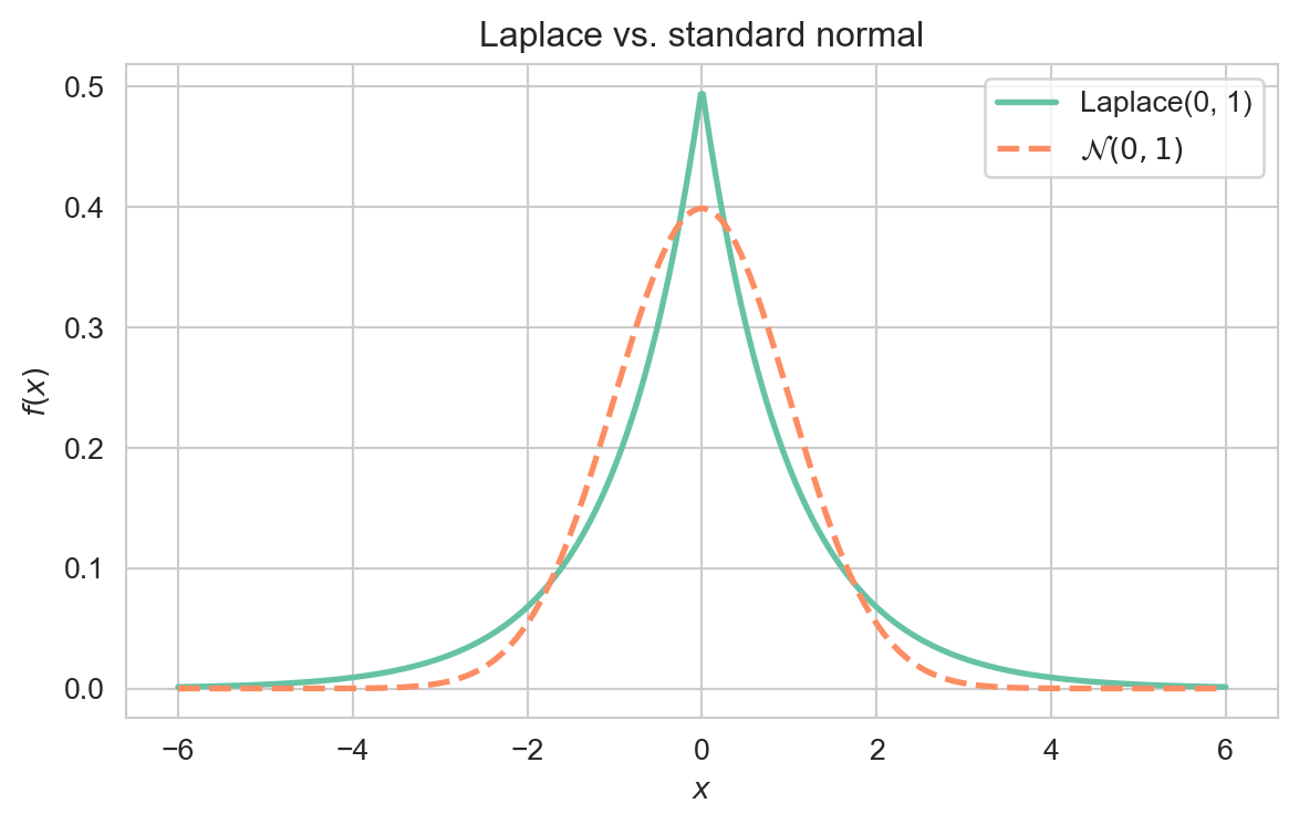
Laplace density (\(\mu = 0\)) compared with the standard normal, showing its sharper peak and heavier tails.

3 Key Properties

The expectation and variance of \(X \sim \text{Laplace}(\mu, b)\) are

\[ \mathbb{E}[X] = \mu \quad \& \quad \operatorname{Var}(X) = 2b^2. \]

Proof. By symmetry of the density about \(\mu\), \(\mathbb{E}[X] = \mu\). Centring at \(\mu\) and using \(\int_0^\infty y^2 e^{-y/b} \, dy = 2b^3\),

\[ \operatorname{Var}(X) = \frac{1}{b}\int_0^\infty y^2 e^{-y/b} \, dy = 2b^2. \]

4 Generating Functions

The moment generating function (MGF) of \(X \sim \text{Laplace}(\mu, b)\) is

\[ M_X(t) = \frac{e^{\mu t}}{1 - b^2 t^2}, \quad |t| < \frac{1}{b}. \]

The characteristic function of \(X \sim \text{Laplace}(\mu, b)\) is

\[ \varphi_X(t) = \frac{e^{i\mu t}}{1 + b^2 t^2}. \]

5 Relationship to Other Distributions

  • Exponential Distribution: If \(Y_1, Y_2 \sim \text{Exponential}(1/b)\) are independent, then \(\mu + Y_1 - Y_2 \sim \text{Laplace}(\mu, b)\).
  • Normal Distribution: A Laplace variable can be written as a normal with an exponentially distributed random variance (a scale mixture), and both are symmetric location-scale families.

6 Examples and Applications

Minimising absolute errors corresponds to maximum-likelihood estimation under Laplace-distributed noise, giving estimators that resist outliers.

A Laplace prior on regression coefficients yields \(\ell_1\) regularisation, encouraging sparse solutions.

Adding Laplace-distributed noise calibrated to a query’s sensitivity is the standard mechanism for achieving differential privacy.
7 Backlinks

Back to top