The exponential distribution is a continuous probability distribution that models the time between consecutive events in a poisson-process. It is the unique continuous distribution with the memoryless property.
A random variable \(X\) follows an exponential distribution with rate parameter \(\lambda > 0\) if
\[
X \sim \text{Exponential}(\lambda) \quad \text{or}
\quad X \sim \mathcal{E}(\lambda).
\]
An alternative parameterisation uses the scale parameter \(\theta = 1/\lambda\).
2 Probability Density Function
The probability density function is
\[
f(x) = \begin{cases}
\lambda e^{-\lambda x} & x \geq 0, \\
0 & x < 0.
\end{cases}
\]
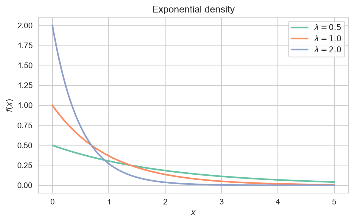
Interpretation: The density decays exponentially, so short waiting times are the most likely and arbitrarily long waits become increasingly rare.
Plotting code
import numpy as npimport matplotlib.pyplot as pltimport seaborn as snsfrom scipy.stats import exponsns.set_style('whitegrid')sns.set_palette('Set2')x = np.linspace(0, 5, 400)fig, ax = plt.subplots(figsize=(7, 4))for lam in (0.5, 1.0, 2.0): ax.plot(x, expon.pdf(x, scale=1/ lam), lw=2, label=rf'$\lambda = {lam}$')ax.set_xlabel('$x$')ax.set_ylabel('$f(x)$')ax.set_title('Exponential density')ax.legend()plt.show()
Density of the exponential distribution for several rate parameters \(\lambda\).
The cumulative distribution function is
\[
F(x) = \begin{cases}
1 - e^{-\lambda x} & x \geq 0, \\
0 & x < 0.
\end{cases}
\]
3 Key Properties
The expectation and variance of \(X \sim \text{Exponential}(\lambda)\) are
The exponential distribution is the unique continuous distribution with the memoryless property: for any \(s, t > 0\),
\[
\mathbb{P}(X > s + t \mid X > s) = \mathbb{P}(X > t).
\]
Proof. Since \(\mathbb{P}(X > u) = e^{-\lambda u}\),
\[
\mathbb{P}(X > s + t \mid X > s)
= \frac{e^{-\lambda(s + t)}}{e^{-\lambda s}}
= e^{-\lambda t} = \mathbb{P}(X > t).
\]
Interpretation: Knowing that an event has not occurred for time \(s\) does not change the distribution of the remaining waiting time.
6 Relationship to Other Distributions
Poisson Distribution: If events follow a poisson-process with rate \(\lambda\), the number of events in \([0, t]\) is \(\text{Poisson}(\lambda t)\) and the inter-arrival times are i.i.d. \(\text{Exponential}(\lambda)\).
Gamma Distribution: A sum of \(n\) i.i.d. \(\text{Exponential}(\lambda)\) variables is \(\text{Gamma}(n, \lambda)\).