Gamma Distribution

Author

John Robin Inston

Published

August 30, 2026

1 Introduction

The Gamma distribution is a two-parameter family of continuous probability distributions that generalises the Exponential Distribution. It arises naturally as the sum of independent exponential random variables and is used to model waiting times, lifetimes, and rates.

A random variable \(X\) follows a Gamma distribution with shape parameter \(\alpha > 0\) and rate parameter \(\beta > 0\) if

\[ X \sim \text{Gamma}(\alpha, \beta) \quad \text{or} \quad X \sim \Gamma(\alpha, \beta). \]

Parameterisations: The shape-rate form uses \(\alpha\) (shape) and \(\beta\) (rate); the shape-scale form uses \(\alpha\) and \(\theta = 1/\beta\) (scale). We use shape-rate here.

2 Probability Density Function

The probability density function (shape-rate form) is

\[ f(x) = \frac{\beta^\alpha}{\Gamma(\alpha)} x^{\alpha - 1} e^{-\beta x}, \quad x > 0, \]

where \(\Gamma(\alpha)\) is the gamma function.

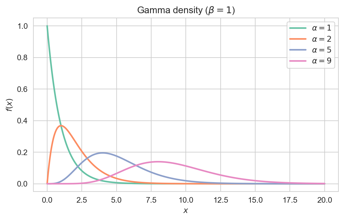
Interpretation: The shape \(\alpha\) controls how peaked the density is and the rate \(\beta\) sets the scale; for \(\alpha \leq 1\) the density is strictly decreasing, and for \(\alpha > 1\) it is unimodal.

Plotting code
import numpy as np
import matplotlib.pyplot as plt
import seaborn as sns
from scipy.stats import gamma

sns.set_style('whitegrid')
sns.set_palette('Set2')

x = np.linspace(0, 20, 400)
fig, ax = plt.subplots(figsize=(7, 4))
for a in (1, 2, 5, 9):
    ax.plot(x, gamma.pdf(x, a, scale=1),
            lw=2, label=rf'$\alpha = {a}$')

ax.set_xlabel('$x$')
ax.set_ylabel('$f(x)$')
ax.set_title(r'Gamma density ($\beta = 1$)')
ax.legend()
plt.show()

Density of the Gamma distribution (rate \(\beta = 1\)) for several shape parameters \(\alpha\).

3 Key Properties

The expectation and variance of \(X \sim \text{Gamma}(\alpha, \beta)\) are

\[ \mathbb{E}[X] = \frac{\alpha}{\beta} \quad \& \quad \operatorname{Var}(X) = \frac{\alpha}{\beta^2}. \]

Proof. Using \(\int_0^\infty x^{\alpha} e^{-\beta x} \, dx = \Gamma(\alpha + 1)/\beta^{\alpha + 1}\),

\[ \mathbb{E}[X] = \frac{\beta^\alpha}{\Gamma(\alpha)} \cdot \frac{\Gamma(\alpha + 1)}{\beta^{\alpha + 1}} = \frac{\alpha}{\beta}. \]

Similarly \(\mathbb{E}[X^2] = \alpha(\alpha + 1)/\beta^2\), so \(\operatorname{Var}(X) = \alpha/\beta^2\).

4 Generating Functions

The moment generating function (MGF) of \(X \sim \text{Gamma}(\alpha, \beta)\) is

\[ M_X(t) = \left(\frac{\beta}{\beta - t}\right)^\alpha, \quad t < \beta. \]

The characteristic function of \(X \sim \text{Gamma}(\alpha, \beta)\) is

\[ \varphi_X(t) = \left(\frac{\beta}{\beta - it}\right)^\alpha. \]

5 Sums of Independent Gamma RVs

If \(X_i \sim \text{Gamma}(\alpha_i, \beta)\) are independent (same rate \(\beta\)), then

\[ \sum_{i=1}^n X_i \sim \text{Gamma}\!\left(\sum_{i=1}^n \alpha_i, \beta\right). \]

Proof. The MGF product gives \(\prod_{i=1}^n (\beta/(\beta - t))^{\alpha_i} = (\beta/(\beta - t))^{\sum_i \alpha_i}\).

In particular, if \(X_1, \ldots, X_n\) are i.i.d. \(\text{Exponential}(\beta)\), then \(X_1 + \cdots + X_n \sim \text{Gamma}(n, \beta)\), so the Gamma distribution models the total of \(n\) independent waiting times.
6 Special Cases and Relationships

  • Exponential Distribution: \(\text{Gamma}(1, \beta) = \text{Exponential}(\beta)\).
  • Erlang: When \(\alpha = n\) is a positive integer, \(\text{Gamma}(n, \beta)\) is the Erlang distribution.
  • Chi-Squared Distribution: \(\text{Gamma}(k/2, 1/2) = \chi^2_k\).
  • Beta Distribution: If \(U \sim \text{Gamma}(\alpha, 1)\) and \(V \sim \text{Gamma}(\beta, 1)\) are independent, then \(\frac{U}{U + V} \sim \text{Beta}(\alpha, \beta)\).

7 Examples and Applications

The total time to wait for \(n\) events in a Poisson process — the sum of \(n\) exponential inter-arrival times — is \(\text{Gamma}(n, \lambda)\).

The lifetime of a system with parallel redundant components can be modelled with a Gamma distribution.

The Gamma distribution is the conjugate prior for the rate parameter of a Poisson or exponential likelihood.

8 Backlinks

Back to top