Beta Distribution – John Robin Inston

1 Introduction

The Beta distribution is a family of continuous probability distributions on the interval \([0, 1]\), controlled by two shape parameters. It is a flexible model for proportions, probabilities, and random variables bounded between \(0\) and \(1\).

A random variable \(X\) follows a Beta distribution with shape parameters \(\alpha > 0\) and \(\beta > 0\) if

\[ X \sim \text{Beta}(\alpha, \beta) \quad \text{or} \quad X \sim B(\alpha, \beta). \]

2 Probability Density Function

The probability density function is

\[ f(x) = \frac{1}{B(\alpha, \beta)} x^{\alpha - 1} (1 - x)^{\beta - 1}, \quad x \in [0, 1], \]

where the beta function is

\[ B(\alpha, \beta) = \frac{\Gamma(\alpha)\Gamma(\beta)} {\Gamma(\alpha + \beta)}. \]

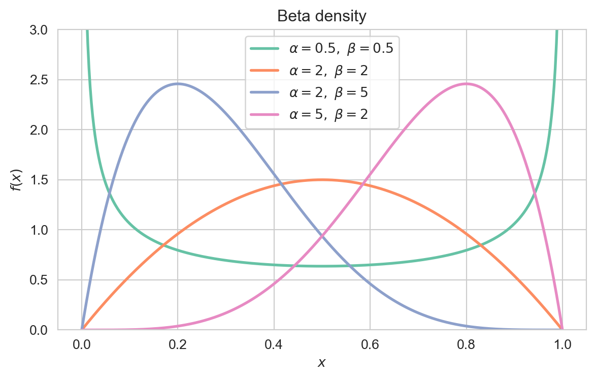
Interpretation: The exponents \(\alpha - 1\) and \(\beta - 1\) pull mass toward \(1\) and \(0\) respectively, giving the distribution its characteristic flexibility on the unit interval.

Plotting code

import numpy as np
import matplotlib.pyplot as plt
import seaborn as sns
from scipy.stats import beta

sns.set_style('whitegrid')
sns.set_palette('Set2')

x = np.linspace(0, 1, 400)
fig, ax = plt.subplots(figsize=(7, 4))
for a, b in ((0.5, 0.5), (2, 2), (2, 5), (5, 2)):
    ax.plot(x, beta.pdf(x, a, b),
            lw=2, label=rf'$\alpha={a},\ \beta={b}$')

ax.set_xlabel('$x$')
ax.set_ylabel('$f(x)$')
ax.set_title('Beta density')
ax.set_ylim(0, 3)
ax.legend()
plt.show()

Density of the Beta distribution for several shape parameter pairs \((\alpha, \beta)\).

3 Key Properties

The expectation and variance of \(X \sim \text{Beta}(\alpha, \beta)\) are

\[ \mathbb{E}[X] = \frac{\alpha}{\alpha + \beta} \quad \& \quad \operatorname{Var}(X) = \frac{\alpha\beta} {(\alpha + \beta)^2(\alpha + \beta + 1)}. \]

Proof. Using \(\int_0^1 x^{\alpha}(1 - x)^{\beta - 1} \, dx = B(\alpha + 1, \beta)\),

\[ \mathbb{E}[X] = \frac{B(\alpha + 1, \beta)}{B(\alpha, \beta)} = \frac{\Gamma(\alpha + 1)\Gamma(\alpha + \beta)} {\Gamma(\alpha)\Gamma(\alpha + \beta + 1)} = \frac{\alpha}{\alpha + \beta}. \]

The variance follows from \(\mathbb{E}[X^2] = \frac{\alpha(\alpha + 1)}{(\alpha + \beta)(\alpha + \beta + 1)}\).

4 Flexibility and Shape

For different parameter values the Beta distribution takes qualitatively different shapes:

\(\alpha = \beta = 1\): uniform on \([0, 1]\).
\(\alpha = \beta > 1\): symmetric, concentrated near \(0.5\).
\(\alpha = \beta < 1\): U-shaped, concentrated near \(0\) and \(1\).
\(\alpha > \beta\): skewed toward \(1\); \(\beta > \alpha\): skewed toward \(0\).

5 Relationship to Other Distributions

Continuous Uniform Distribution: \(\text{Beta}(1, 1) = U(0, 1)\), and Beta arises as the distribution of uniform order statistics.
Binomial Distribution: The conjugate prior for the success probability \(p\); a \(\text{Beta}(\alpha, \beta)\) prior with \(k\) successes in \(n\) trials gives a \(\text{Beta}(k + \alpha, n - k + \beta)\) posterior.
Gamma Distribution: If \(U \sim \text{Gamma}(\alpha, 1)\) and \(V \sim \text{Gamma}(\beta, 1)\) are independent, then \(\frac{U}{U + V} \sim \text{Beta}(\alpha, \beta)\).
Dirichlet Distribution: The multivariate generalisation of the Beta distribution to the probability simplex.

6 Examples and Applications

The unknown fraction of website visitors who make a purchase can be modelled with a Beta prior and updated as data arrive.

A Beta distribution represents prior belief about the proportion of voters supporting a candidate before any polling data are collected.

In PERT analysis, task completion ratios and durations are modelled with Beta distributions to capture bounded uncertainty.