Continuous Uniform Distribution

1 Introduction

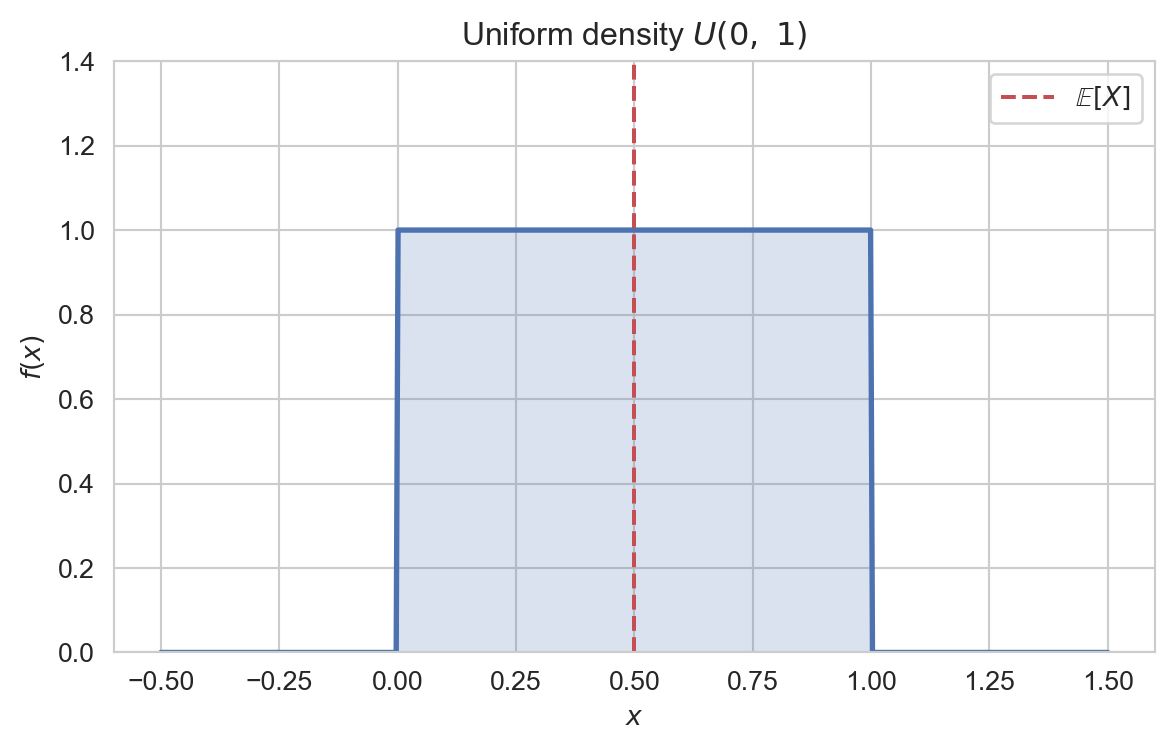
The continuous uniform distribution is a continuous probability distribution in which all outcomes in a bounded interval are equally likely. It is the simplest continuous distribution and the continuous analogue of the Discrete Uniform Distribution.

A random variable \(X\) follows a continuous uniform distribution on the interval \([a, b]\) with \(a < b\) if

\[ X \sim \text{Uniform}(a, b) \quad \text{or} \quad X \sim U(a, b). \]

The most common case is the standard uniform distribution on \([0, 1]\), denoted \(U(0, 1)\).

2 Probability Density Function

The probability density function is

\[ f(x) = \begin{cases} \dfrac{1}{b - a} & x \in [a, b], \\[4pt] 0 & \text{otherwise.} \end{cases} \]

Interpretation: The constant value \(\frac{1}{b-a}\) ensures that the density integrates to \(1\) over \([a, b]\); no value in the interval is preferred over any other.

Plotting code

import numpy as np
import matplotlib.pyplot as plt
import seaborn as sns

sns.set_style('whitegrid')
sns.set_palette('Set2')

a, b = 0.0, 1.0
x = np.linspace(a - 0.5, b + 0.5, 500)
y = np.where((x >= a) & (x <= b), 1 / (b - a), 0.0)

fig, ax = plt.subplots(figsize=(7, 4))
ax.plot(x, y, color='#4c72b0', lw=2)
ax.fill_between(x, y, color='#4c72b0', alpha=0.2)
ax.axvline((a + b) / 2, color='#c44e52', ls='--', lw=1.5,
           label=r'$\mathbb{E}[X]$')

ax.set_xlabel('$x$')
ax.set_ylabel('$f(x)$')
ax.set_title(r'Uniform density $U(0,\ 1)$')
ax.set_ylim(0, 1.4)
ax.legend()
plt.show()

Density of the standard uniform \(U(0, 1)\).

The cumulative distribution function is

\[ F(x) = \begin{cases} 0 & x < a, \\[2pt] \dfrac{x - a}{b - a} & a \leq x \leq b, \\[4pt] 1 & x > b. \end{cases} \]

3 Key Properties

The expectation and variance of \(X \sim \text{Uniform}(a, b)\) are

\[ \mathbb{E}[X] = \frac{a + b}{2} \quad \& \quad \operatorname{Var}(X) = \frac{(b - a)^2}{12}. \]

Proof. Directly,

\[ \mathbb{E}[X] = \int_a^b \frac{x}{b - a} \, dx = \frac{b^2 - a^2}{2(b - a)} = \frac{a + b}{2}. \]

Since \(\mathbb{E}[X^2] = \frac{a^2 + ab + b^2}{3}\),

\[ \operatorname{Var}(X) = \frac{a^2 + ab + b^2}{3} - \frac{(a + b)^2}{4} = \frac{(b - a)^2}{12}. \]

4 Generating Functions

The moment generating function (MGF) of \(X \sim \text{Uniform}(a, b)\) is

\[ M_X(t) = \frac{e^{tb} - e^{ta}}{t(b - a)}, \quad t \neq 0, \]

with \(M_X(0) = 1\).

The characteristic function of \(X \sim \text{Uniform}(a, b)\) is

\[ \varphi_X(t) = \frac{e^{itb} - e^{ita}}{it(b - a)}, \quad t \neq 0. \]

5 Affine Transformations and Order Statistics

If \(X \sim \text{Uniform}(a, b)\) and \(Y = cX + d\) with \(c > 0\), then

\[ Y \sim \text{Uniform}(ca + d, cb + d). \]

In particular, if \(X \sim U(0, 1)\) then \((b - a)X + a \sim U(a, b)\).

If \(U_1, \ldots, U_n\) are i.i.d. \(U(0, 1)\) with order statistics \(U_{(1)} \leq \cdots \leq U_{(n)}\), then the \(k\)-th order statistic follows a Beta Distribution:

\[ U_{(k)} \sim \text{Beta}(k, n + 1 - k). \]

6 Relationship to Other Distributions

Discrete Uniform Distribution: The discrete analogue on a finite set of equally likely values.
Beta Distribution: \(U(0, 1) = \text{Beta}(1, 1)\), and order statistics of uniforms are Beta distributed.
Inverse transform sampling: If \(F\) is a continuous CDF and \(U \sim U(0, 1)\), then \(F^{-1}(U)\) has distribution \(F\) — the basis for simulating any Random Variable Transformations.

7 Examples and Applications

\(U(0, 1)\) is the foundation for generating samples from any distribution via inverse transform sampling.

If an event is equally likely to occur at any time in a fixed window, its arrival time is modelled as \(\text{Uniform}(a, b)\).

A measurement known only to lie within a specified tolerance band, with no further information, is often modelled as uniform over that band.