Discrete Uniform Distribution – John Robin Inston

1 Introduction

The discrete uniform distribution is a discrete probability distribution in which a finite number of equally likely outcomes each occur with the same probability. It is the discrete analogue of the Continuous Uniform Distribution.

A random variable \(X\) follows a discrete uniform distribution on the set \(\{1, 2, \ldots, n\}\) if

\[ X \sim \text{DiscreteUniform}(n) \quad \text{or} \quad X \sim \mathcal{U}\{1, \ldots, n\}. \]

2 Probability Mass Function

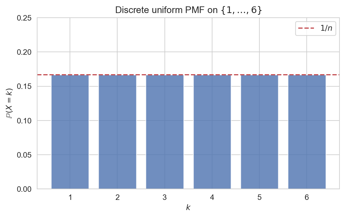
The probability mass function is

\[ \mathbb{P}(X = k) = \frac{1}{n}, \quad k \in \{1, 2, \ldots, n\}. \]

Interpretation: Every one of the \(n\) outcomes is equally likely, so the distribution encodes complete indifference between them.

Plotting code

import numpy as np
import matplotlib.pyplot as plt
import seaborn as sns

sns.set_style('whitegrid')
sns.set_palette('Set2')

n = 6
k = np.arange(1, n + 1)
pmf = np.full(n, 1 / n)

fig, ax = plt.subplots(figsize=(7, 4))
ax.bar(k, pmf, color='#4c72b0', alpha=0.8)
ax.axhline(1 / n, color='#c44e52', ls='--', lw=1.5,
           label=r'$1/n$')

ax.set_xlabel('$k$')
ax.set_ylabel(r'$\mathbb{P}(X = k)$')
ax.set_title(r'Discrete uniform PMF on $\{1, \ldots, 6\}$')
ax.set_ylim(0, 0.25)
ax.legend()
plt.show()

Probability mass function of a discrete uniform distribution on \(\{1, \ldots, 6\}\) (a fair die).

3 Key Properties

The expectation and variance of \(X \sim \text{DiscreteUniform}(n)\) are

\[ \mathbb{E}[X] = \frac{n+1}{2} \quad \& \quad \operatorname{Var}(X) = \frac{n^2 - 1}{12}. \]

Proof. Using \(\sum_{k=1}^n k = \frac{n(n+1)}{2}\),

\[ \mathbb{E}[X] = \frac{1}{n} \sum_{k=1}^n k = \frac{n+1}{2}. \]

Using \(\sum_{k=1}^n k^2 = \frac{n(n+1)(2n+1)}{6}\) gives \(\mathbb{E}[X^2] = \frac{(n+1)(2n+1)}{6}\), hence

\[ \operatorname{Var}(X) = \frac{(n+1)(2n+1)}{6} - \left(\frac{n+1}{2}\right)^2 = \frac{n^2 - 1}{12}. \]

4 Generating Functions

The probability generating function (PGF) of \(X \sim \text{DiscreteUniform}(n)\) is

\[ G_X(s) = \frac{1}{n} \sum_{k=1}^n s^k = \frac{s(1 - s^n)}{n(1 - s)}, \quad s \neq 1. \]

The moment generating function (MGF) of \(X \sim \text{DiscreteUniform}(n)\) is

\[ M_X(t) = \frac{1}{n} \sum_{k=1}^n e^{tk} = \frac{e^t(1 - e^{nt})}{n(1 - e^t)}, \quad t \neq 0. \]

5 General Support

More generally, \(X\) may be uniform on \(\{a, a+1, \ldots, b\}\) with \(n = b - a + 1\) equally likely values. Then

\[ \mathbb{E}[X] = \frac{a+b}{2} \quad \& \quad \operatorname{Var}(X) = \frac{(b - a + 1)^2 - 1}{12}. \]

6 Relationship to Other Distributions

Continuous Uniform Distribution: The continuous analogue on an interval \([a, b]\).
Binomial Distribution: A fair Bernoulli trial is the special case \(\text{DiscreteUniform}(2)\) shifted to \(\{0, 1\}\).
Sampling a value uniformly from \(\{1, \ldots, n\}\) underlies many randomised algorithms and simulation methods.

7 Examples and Applications

The outcome of rolling a fair six-sided die is \(X \sim \text{DiscreteUniform}(6)\), with \(\mathbb{E}[X] = 3.5\).

Selecting one card position uniformly at random from a shuffled deck of \(52\) cards is \(X \sim \text{DiscreteUniform}(52)\).

Pseudo-random integer generators return values that are (approximately) discrete uniform over a fixed range, forming a building block for simulation.