Binomial Distribution – John Robin Inston

1 Introduction

The binomial distribution is a discrete probability distribution that models the number of successes in a fixed number of independent trials, each with the same probability of success.

A random variable \(X\) follows a binomial distribution with parameters \(n\) (number of trials) and \(p\) (probability of success) if

\[ X \sim \text{Binomial}(n, p) \quad \text{or} \quad X \sim \mathcal{B}(n, p). \]

2 Probability Mass Function

The probability mass function is

\[ \mathbb{P}(X = k) = \binom{n}{k} p^k (1-p)^{n-k}, \quad k \in \{0, 1, \ldots, n\}. \]

Interpretation: We choose \(k\) positions out of \(n\) trials for successes (\(\binom{n}{k}\) ways), then assign probability \(p^k\) to these successes and \((1-p)^{n-k}\) to the remaining failures.

Special case: When \(n = 1\) we recover the Bernoulli distribution, with \(\mathbb{P}(X = 1) = p\) and \(\mathbb{P}(X = 0) = 1 - p\).

Plotting code

import numpy as np
import matplotlib.pyplot as plt
import seaborn as sns
from scipy.stats import binom

sns.set_style('whitegrid')
sns.set_palette('Set2')

n, p = 20, 0.3
k = np.arange(0, n + 1)
pmf = binom.pmf(k, n, p)

fig, ax = plt.subplots(figsize=(7, 4))
ax.bar(k, pmf, color='#4c72b0', alpha=0.8)
ax.axvline(n * p, color='#c44e52', ls='--', lw=1.5,
           label=r'$\mathbb{E}[X] = np$')

ax.set_xlabel('$k$')
ax.set_ylabel(r'$\mathbb{P}(X = k)$')
ax.set_title(r'Binomial PMF $\mathcal{B}(20,\ 0.3)$')
ax.legend()
plt.show()

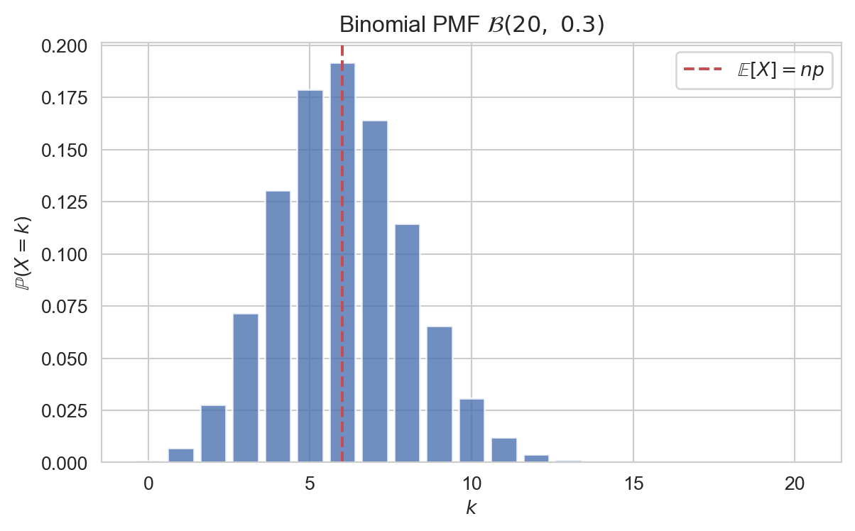
Probability mass function of \(\text{Binomial}(20, 0.3)\).

3 Key Properties

The expectation and variance of \(X \sim \text{Binomial}(n, p)\) are

\[ \mathbb{E}[X] = np \quad \& \quad \operatorname{Var}(X) = np(1-p). \]

Proof. Write \(X = X_1 + X_2 + \cdots + X_n\) where each \(X_i \sim \text{Bernoulli}(p)\) is independent. Then

\[ \mathbb{E}[X] = \sum_{i=1}^n \mathbb{E}[X_i] = np, \]

and by independence

\[ \operatorname{Var}(X) = \sum_{i=1}^n \operatorname{Var}(X_i) = n \cdot p(1-p). \]

4 Generating Functions

The binomial distribution has several Generating Functions that follow directly from its representation as a sum of Bernoulli trials.

The probability generating function (PGF) of \(X \sim \text{Binomial}(n, p)\) is

\[ G_X(s) = (1 - p + ps)^n. \]

The moment generating function (MGF) of \(X \sim \text{Binomial}(n, p)\) is

\[ M_X(t) = (1 - p + pe^t)^n. \]

The characteristic function of \(X \sim \text{Binomial}(n, p)\) is

\[ \varphi_X(t) = (1 - p + pe^{it})^n. \]

5 Sums of Independent Binomial RVs

If \(X \sim \text{Binomial}(n_1, p)\) and \(Y \sim \text{Binomial}(n_2, p)\) are independent (same \(p\)), then

\[ X + Y \sim \text{Binomial}(n_1 + n_2, p). \]

Proof. The MGF product gives \((1 - p + pe^t)^{n_1} \cdot (1 - p + pe^t)^{n_2} = (1 - p + pe^t)^{n_1 + n_2}\).

6 Relationship to Other Distributions

Normal Distribution: For large \(n\), \(\frac{X - np}{\sqrt{np(1 - p)}} \xrightarrow{d} \mathcal{N}(0, 1)\) (de Moivre–Laplace theorem).
Poisson Distribution: If \(n \to \infty\) and \(p \to 0\) with \(np = \lambda\) fixed, then \(X \xrightarrow{d} \text{Poisson}(\lambda)\).
Geometric Distribution: Models the number of trials until the first success in the same sequence of Bernoulli trials.
Beta Distribution: The conjugate prior for the success probability \(p\) in Bayesian inference.

7 Examples and Applications

The number of heads in \(10\) fair coin flips is \(X \sim \text{Binomial}(10, 0.5)\), with \(\mathbb{E}[X] = 5\).

The number of defective items in a batch of \(100\) when the defect rate is \(2\%\) is \(X \sim \text{Binomial}(100, 0.02)\).

The number of patients recovering from a treatment applied to \(50\) people with success rate \(80\%\) is \(X \sim \text{Binomial}(50, 0.8)\).