Geometric Distribution – John Robin Inston

1 Introduction

The geometric distribution is a discrete probability distribution that models the number of independent Bernoulli trials needed to obtain the first success. It is the discrete distribution with the memoryless property, mirroring the Exponential Distribution in continuous time.

A random variable \(X\) follows a geometric distribution with success probability \(p \in (0, 1]\) if it counts the trial on which the first success occurs,

\[ X \sim \text{Geometric}(p). \]

2 Probability Mass Function

The probability mass function is

\[ \mathbb{P}(X = k) = (1 - p)^{k-1} p, \quad k \in \{1, 2, 3, \ldots\}. \]

Interpretation: The first \(k - 1\) trials are failures, each with probability \(1 - p\), followed by a success with probability \(p\). An alternative convention counts the number of failures before the first success, supported on \(\{0, 1, 2, \ldots\}\).

Plotting code

import numpy as np
import matplotlib.pyplot as plt
import seaborn as sns
from scipy.stats import geom

sns.set_style('whitegrid')
sns.set_palette('Set2')

p = 0.4
k = np.arange(1, 16)
pmf = geom.pmf(k, p)

fig, ax = plt.subplots(figsize=(7, 4))
ax.bar(k, pmf, color='#4c72b0', alpha=0.8)
ax.axvline(1 / p, color='#c44e52', ls='--', lw=1.5,
           label=r'$\mathbb{E}[X] = 1/p$')

ax.set_xlabel('$k$')
ax.set_ylabel(r'$\mathbb{P}(X = k)$')
ax.set_title(r'Geometric PMF ($p = 0.4$)')
ax.legend()
plt.show()

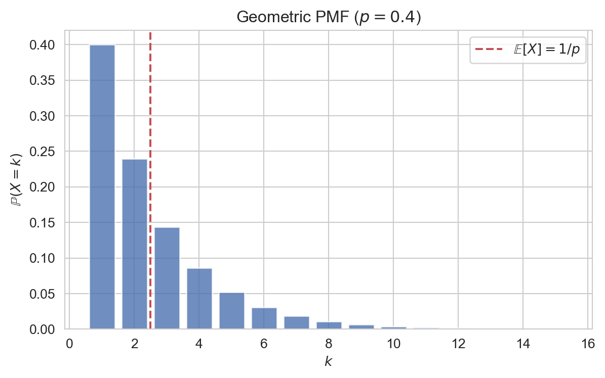
Probability mass function of \(\text{Geometric}(0.4)\) (trials until the first success).

3 Key Properties

The expectation and variance of \(X \sim \text{Geometric}(p)\) are

\[ \mathbb{E}[X] = \frac{1}{p} \quad \& \quad \operatorname{Var}(X) = \frac{1 - p}{p^2}. \]

Proof. Differentiating the geometric series \(\sum_{k=1}^\infty (1-p)^{k-1} = 1/p\) term by term,

\[ \mathbb{E}[X] = \sum_{k=1}^\infty k (1-p)^{k-1} p = p \cdot \frac{1}{p^2} = \frac{1}{p}. \]

A second differentiation gives \(\mathbb{E}[X(X-1)] = 2(1-p)/p^2\), so \(\operatorname{Var}(X) = (1-p)/p^2\).

4 The Memoryless Property

The geometric distribution is the unique discrete distribution with the memoryless property: for all \(s, t \in \{0, 1, 2, \ldots\}\),

\[ \mathbb{P}(X > s + t \mid X > s) = \mathbb{P}(X > t). \]

Proof. Since \(\mathbb{P}(X > m) = (1-p)^m\),

\[ \mathbb{P}(X > s + t \mid X > s) = \frac{(1-p)^{s+t}}{(1-p)^s} = (1-p)^t = \mathbb{P}(X > t). \]

5 Generating Functions

The probability generating function (PGF) of \(X \sim \text{Geometric}(p)\) is

\[ G_X(s) = \frac{ps}{1 - (1 - p)s}, \quad |s| < \frac{1}{1 - p}. \]

The moment generating function (MGF) of \(X \sim \text{Geometric}(p)\) is

\[ M_X(t) = \frac{pe^t}{1 - (1 - p)e^t}, \quad t < -\ln(1 - p). \]

6 Relationship to Other Distributions

Exponential Distribution: The continuous analogue; both are the unique memoryless distributions in their respective settings.
Binomial Distribution: Both arise from sequences of independent Bernoulli trials — binomial counts successes in \(n\) trials, geometric counts trials until the first success.
Negative binomial: The number of trials until the \(r\)-th success is a sum of \(r\) independent geometric random variables.

7 Examples and Applications

The number of fair coin flips until the first head is \(X \sim \text{Geometric}(0.5)\), with \(\mathbb{E}[X] = 2\).

The number of independent attempts until a machine first fails, when each attempt fails with probability \(p\), is geometrically distributed.

The position of the first defective item on a production line, when each item is independently defective with probability \(p\), follows \(\text{Geometric}(p)\).