The \(F\)-distribution is a continuous probability distribution that arises as the ratio of two independent Chi-Squared Distribution variables, each divided by its degrees of freedom. It is central to the analysis of variance (ANOVA) and to tests comparing two variances.
A random variable \(X\) follows an \(F\)-distribution with \(d_1\) and \(d_2\) degrees of freedom if
\[
X \sim F_{d_1, d_2} \quad \text{or} \quad X \sim F(d_1, d_2).
\]
2 Construction from Chi-Squared
If \(U \sim \chi^2_{d_1}\) and \(V \sim \chi^2_{d_2}\) are independent, then
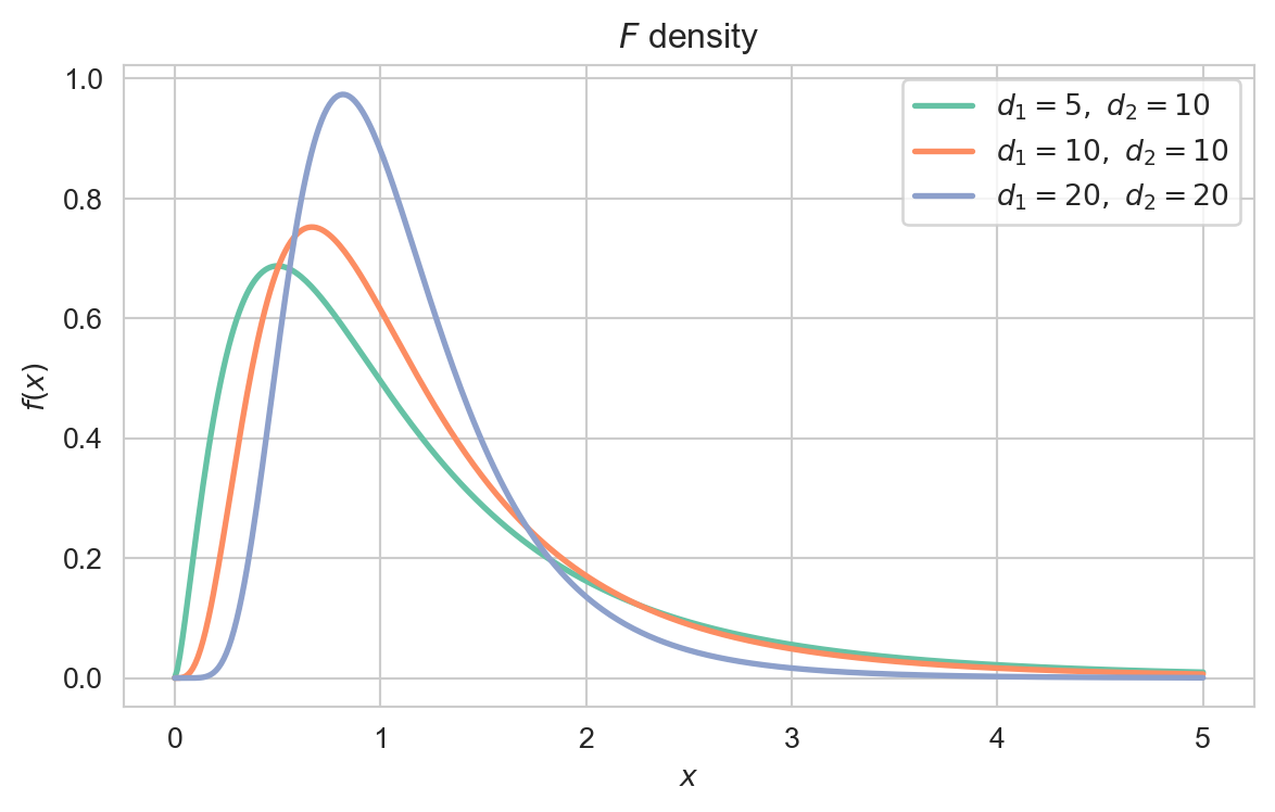
Interpretation: Values near \(1\) are typical when the two underlying variances are comparable; large values indicate the numerator variance dominates.
Plotting code
import numpy as npimport matplotlib.pyplot as pltimport seaborn as snsfrom scipy.stats import f as fdistsns.set_style('whitegrid')sns.set_palette('Set2')x = np.linspace(0, 5, 400)fig, ax = plt.subplots(figsize=(7, 4))for d1, d2 in ((5, 10), (10, 10), (20, 20)): ax.plot(x, fdist.pdf(x, d1, d2), lw=2, label=rf'$d_1={d1},\ d_2={d2}$')ax.set_xlabel('$x$')ax.set_ylabel('$f(x)$')ax.set_title('$F$ density')ax.legend()plt.show()
Density of the \(F\)-distribution for several pairs of degrees of freedom \((d_1, d_2)\).
Proof. Write \(X = (U/d_1)/(V/d_2)\) with \(U \sim \chi^2_{d_1}\), \(V \sim \chi^2_{d_2}\) independent. Then \(\mathbb{E}[X] =
\frac{d_2}{d_1}\mathbb{E}[U]\,\mathbb{E}[V^{-1}]\). Using \(\mathbb{E}[U] = d_1\) and \(\mathbb{E}[V^{-1}] = 1/(d_2 - 2)\) gives \(\mathbb{E}[X] = d_2/(d_2 - 2)\). The variance follows from the second inverse moment of \(V\).
Beta Distribution: If \(X \sim F_{d_1, d_2}\), then \(\frac{d_1 X}{d_1 X + d_2} \sim \text{Beta}(d_1/2, d_2/2)\).
Reciprocal: If \(X \sim F_{d_1, d_2}\) then \(1/X \sim F_{d_2, d_1}\).
6 Examples and Applications
In one-way ANOVA the ratio of between-group to within-group mean squares follows an \(F\)-distribution under the null hypothesis of equal group means.
The ratio \(S_1^2 / S_2^2\) of two independent normal sample variances is \(F\)-distributed, giving a test of the hypothesis \(\sigma_1^2 =
\sigma_2^2\).
The overall \(F\)-test in linear regression compares a fitted model against the intercept-only model to assess joint significance of the predictors.