Chi-Squared Distribution

Author

John Robin Inston

Published

August 30, 2026

1 Introduction

The chi-squared distribution is a continuous probability distribution that arises as the sum of squares of independent standard normal random variables. It is fundamental to hypothesis testing, confidence intervals, and goodness-of-fit tests.

A random variable \(X\) follows a chi-squared distribution with \(k\) degrees of freedom if

\[ X \sim \chi^2_k \quad \text{or} \quad X \sim \chi^2(k). \]

It is a special case of the Gamma Distribution:

\[ \chi^2_k = \text{Gamma}\!\left(\frac{k}{2}, \frac{1}{2}\right). \]

2 Probability Density Function

Using the gamma representation, the probability density function is

\[ f(x) = \frac{1}{2^{k/2}\Gamma(k/2)} x^{k/2 - 1} e^{-x/2}, \quad x > 0. \]

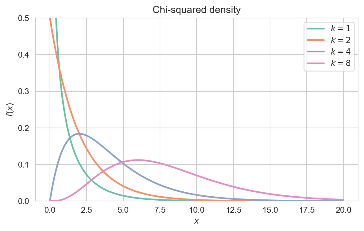
Interpretation: For \(k = 1, 2\) the density is decreasing, while for \(k \geq 3\) it is unimodal and increasingly symmetric as \(k\) grows.

Plotting code
import numpy as np
import matplotlib.pyplot as plt
import seaborn as sns
from scipy.stats import chi2

sns.set_style('whitegrid')
sns.set_palette('Set2')

x = np.linspace(0, 20, 400)
fig, ax = plt.subplots(figsize=(7, 4))
for k in (1, 2, 4, 8):
    ax.plot(x, chi2.pdf(x, k), lw=2, label=rf'$k = {k}$')

ax.set_xlabel('$x$')
ax.set_ylabel('$f(x)$')
ax.set_title('Chi-squared density')
ax.set_ylim(0, 0.5)
ax.legend()
plt.show()

Density of the chi-squared distribution for several degrees of freedom \(k\).

3 Key Properties

The expectation and variance of \(X \sim \chi^2_k\) are

\[ \mathbb{E}[X] = k \quad \& \quad \operatorname{Var}(X) = 2k. \]

Proof. Using the gamma representation with shape \(k/2\) and rate \(1/2\),

\[ \mathbb{E}[X] = \frac{k/2}{1/2} = k, \qquad \operatorname{Var}(X) = \frac{k/2}{(1/2)^2} = 2k. \]

4 Generating Functions

The moment generating function (MGF) of \(X \sim \chi^2_k\) is

\[ M_X(t) = (1 - 2t)^{-k/2}, \quad t < \frac{1}{2}. \]

The characteristic function of \(X \sim \chi^2_k\) is

\[ \varphi_X(t) = (1 - 2it)^{-k/2}. \]

5 Definition via Standard Normals

If \(Z_1, \ldots, Z_k\) are i.i.d. \(\mathcal{N}(0, 1)\), then

\[ X = \sum_{i=1}^k Z_i^2 \sim \chi^2_k. \]

Proof. Each \(Z_i^2 \sim \chi^2_1 = \text{Gamma}(1/2, 1/2)\). By additivity of the Gamma Distribution with common rate, the sum is \(\text{Gamma}(k/2, 1/2) = \chi^2_k\).

If \(X_i \sim \chi^2_{k_i}\) are independent, then
\[ \sum_{i=1}^n X_i \sim \chi^2_{k_1 + \cdots + k_n}. \]

6 Relationship to Other Distributions

  • Gamma Distribution: \(\chi^2_k = \text{Gamma}(k/2, 1/2)\).
  • Normal Distribution: A sum of squared standard normals; and as \(k \to \infty\), \(\frac{X - k}{\sqrt{2k}} \xrightarrow{d} \mathcal{N}(0, 1)\).
  • Student's t-Distribution: A standard normal divided by \(\sqrt{X/k}\) is Student’s \(t\) with \(k\) degrees of freedom.
  • F-Distribution: A ratio of two independent chi-squared variables, each divided by its degrees of freedom, is \(F\)-distributed.

7 Statistical Applications

The chi-squared statistic compares observed and expected frequencies to test whether data follow a hypothesised distribution.

For a normal sample, \(\frac{(n - 1)S^2}{\sigma^2} \sim \chi^2_{n-1}\), which yields confidence intervals and tests for the population variance.

In a contingency table, the chi-squared test assesses whether two categorical variables are independent.

8 Backlinks

Back to top