Student’s t-Distribution – John Robin Inston

1 Introduction

Student’s \(t\)-distribution is a continuous probability distribution that arises when estimating the mean of a normally distributed population from a small sample with unknown variance. It is symmetric and bell-shaped like the Normal Distribution, but with heavier tails.

A random variable \(T\) follows a Student’s \(t\)-distribution with \(\nu > 0\) degrees of freedom if

\[ T \sim t_\nu \quad \text{or} \quad T \sim t(\nu). \]

2 Construction from Normal and Chi-Squared

If \(Z \sim \mathcal{N}(0, 1)\) and \(V \sim \chi^2_\nu\) are independent, then

\[ T = \frac{Z}{\sqrt{V/\nu}} \sim t_\nu. \]

This links the Normal Distribution and the Chi-Squared Distribution: the numerator is a standard normal and the denominator rescales by an independent chi-squared.

3 Probability Density Function

The probability density function is

\[ f(t) = \frac{\Gamma\!\left(\frac{\nu + 1}{2}\right)} {\sqrt{\nu\pi}\,\Gamma\!\left(\frac{\nu}{2}\right)} \left(1 + \frac{t^2}{\nu}\right)^{-\frac{\nu + 1}{2}}, \quad t \in \mathbb{R}. \]

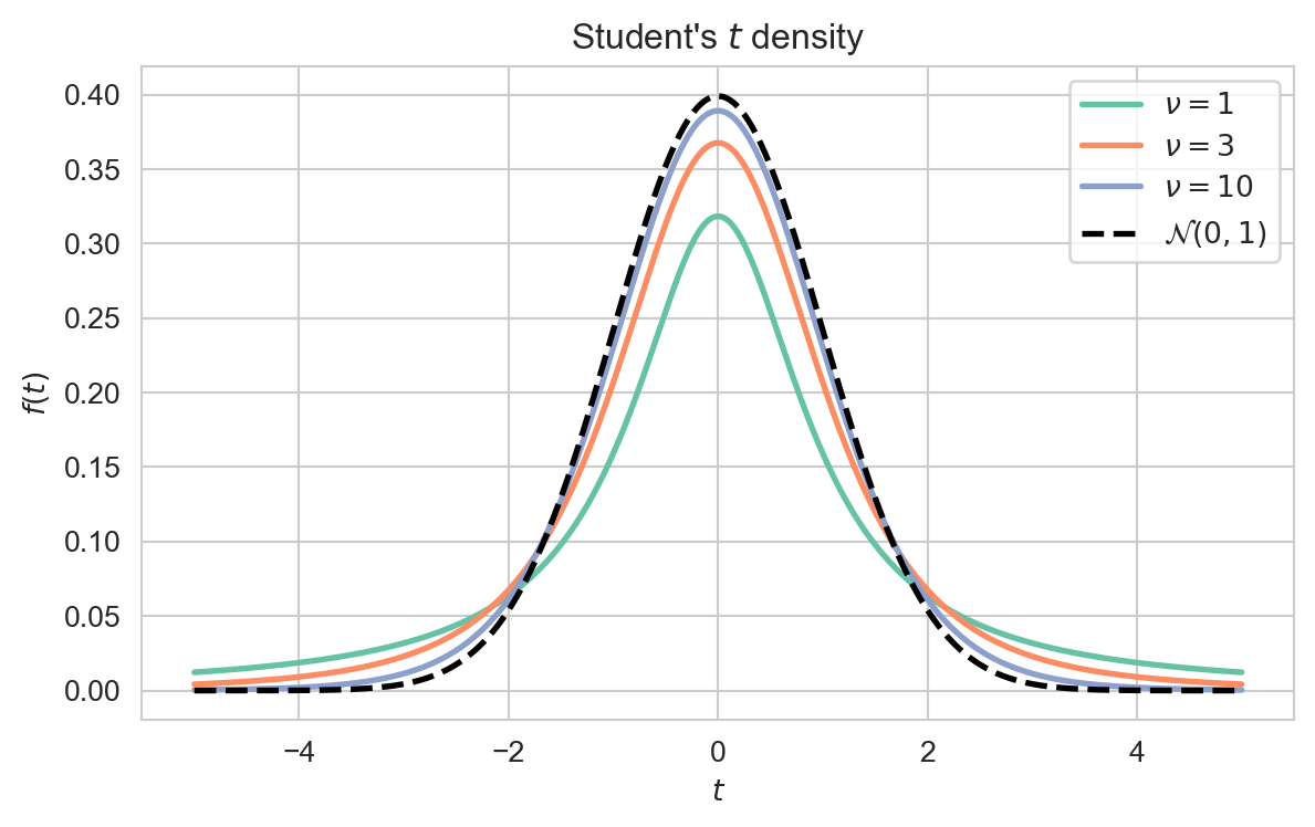
Interpretation: Smaller \(\nu\) gives heavier tails; as \(\nu\) increases the density tightens toward the standard normal.

Plotting code

import numpy as np
import matplotlib.pyplot as plt
import seaborn as sns
from scipy.stats import t as tdist, norm

sns.set_style('whitegrid')
sns.set_palette('Set2')

x = np.linspace(-5, 5, 500)
fig, ax = plt.subplots(figsize=(7, 4))
for nu in (1, 3, 10):
    ax.plot(x, tdist.pdf(x, nu), lw=2, label=rf'$\nu = {nu}$')
ax.plot(x, norm.pdf(x), lw=2, ls='--', color='black',
        label=r'$\mathcal{N}(0, 1)$')

ax.set_xlabel('$t$')
ax.set_ylabel('$f(t)$')
ax.set_title("Student's $t$ density")
ax.legend()
plt.show()

Student’s \(t\) density for several degrees of freedom \(\nu\), with the standard normal limit shown dashed.

4 Key Properties

For \(T \sim t_\nu\),

\[ \mathbb{E}[T] = 0 \ \ (\nu > 1), \qquad \operatorname{Var}(T) = \frac{\nu}{\nu - 2} \ \ (\nu > 2). \]

The mean is undefined for \(\nu \leq 1\) and the variance is infinite for \(1 < \nu \leq 2\).

Proof. The density is even, so whenever the mean exists it is \(0\) by symmetry. For \(\nu > 2\) the second moment follows from the chi-squared representation and the identity \(\mathbb{E}[V^{-1}] = 1/(\nu - 2)\) for \(V \sim \chi^2_\nu\), giving \(\operatorname{Var}(T) = \nu/(\nu - 2)\).

The moment generating function does not exist, because the tails are too heavy for \(\mathbb{E}[e^{sT}]\) to converge for any \(s \neq 0\).

5 Relationship to Other Distributions

Cauchy Distribution: \(t_1\) is the standard Cauchy distribution.
Normal Distribution: As \(\nu \to \infty\), \(t_\nu \xrightarrow{d} \mathcal{N}(0, 1)\).
Chi-Squared Distribution: \(T^2 \sim F_{1, \nu}\), an F-Distribution with \(1\) and \(\nu\) degrees of freedom.

6 Examples and Applications

For a normal sample of size \(n\), the statistic \(\frac{\bar{X} - \mu}{S/\sqrt{n}} \sim t_{n-1}\), which underlies confidence intervals and hypothesis tests for the mean when the variance is unknown.

With few observations the \(t\)-distribution’s heavier tails give wider, more honest confidence intervals than the normal approximation.

Replacing normal errors with \(t\)-distributed errors yields regression models that are less sensitive to outliers.