Rayleigh Distribution

Author

John Robin Inston

Published

August 30, 2026

1 Introduction

The Rayleigh distribution is a continuous probability distribution for the magnitude of a two-dimensional vector whose components are independent, zero-mean normal variables. It arises for wind speeds, signal envelopes, and scattering amplitudes.

A random variable \(X\) follows a Rayleigh distribution with scale parameter \(\sigma > 0\) if

\[ X \sim \text{Rayleigh}(\sigma). \]

2 Probability Density Function

The probability density function is

\[ f(x) = \frac{x}{\sigma^2} \exp\!\left(-\frac{x^2}{2\sigma^2}\right), \quad x \geq 0. \]

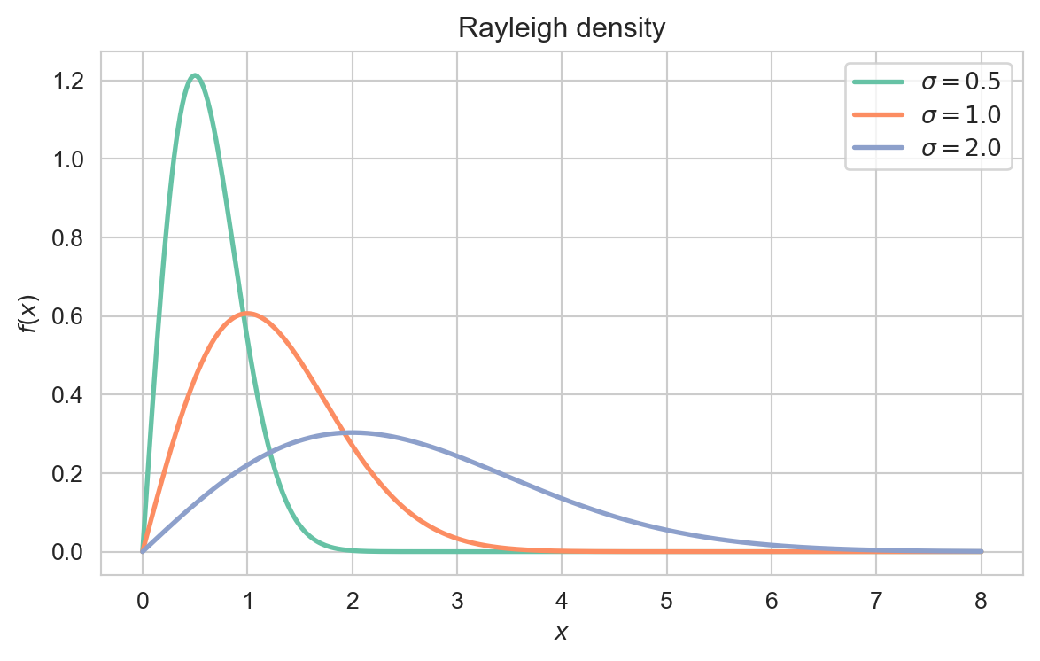
Interpretation: The density vanishes at the origin, rises to a mode at \(x = \sigma\), and then decays like a Gaussian tail.

Plotting code
import numpy as np
import matplotlib.pyplot as plt
import seaborn as sns
from scipy.stats import rayleigh

sns.set_style('whitegrid')
sns.set_palette('Set2')

x = np.linspace(0, 8, 400)
fig, ax = plt.subplots(figsize=(7, 4))
for sigma in (0.5, 1.0, 2.0):
    ax.plot(x, rayleigh.pdf(x, scale=sigma),
            lw=2, label=rf'$\sigma = {sigma}$')

ax.set_xlabel('$x$')
ax.set_ylabel('$f(x)$')
ax.set_title('Rayleigh density')
ax.legend()
plt.show()

Density of the Rayleigh distribution for several scale parameters \(\sigma\).
The cumulative distribution function is

\[ F(x) = 1 - \exp\!\left(-\frac{x^2}{2\sigma^2}\right), \quad x \geq 0. \]

3 Key Properties

For \(X \sim \text{Rayleigh}(\sigma)\),

\[ \mathbb{E}[X] = \sigma\sqrt{\frac{\pi}{2}} \quad \& \quad \operatorname{Var}(X) = \frac{4 - \pi}{2}\sigma^2. \]

Proof. With the substitution \(u = x^2/(2\sigma^2)\),

\[ \mathbb{E}[X] = \int_0^\infty \frac{x^2}{\sigma^2} e^{-x^2/(2\sigma^2)} \, dx = \sigma\sqrt{\frac{\pi}{2}}. \]

Since \(\mathbb{E}[X^2] = 2\sigma^2\), the variance is \(2\sigma^2 - \frac{\pi}{2}\sigma^2 = \frac{4 - \pi}{2}\sigma^2\).

4 Relationship to Other Distributions

5 Examples and Applications

The envelope of a narrowband noise signal, and fading amplitudes in wireless communication, follow a Rayleigh distribution.

Wind speed magnitudes are often modelled as Rayleigh, the special case of the Weibull wind-speed model with shape \(2\).

The distance from the origin to a point with independent normal coordinate errors is Rayleigh distributed, relevant to targeting and navigation.

6 Backlinks

Back to top