Weibull Distribution – John Robin Inston

1 Introduction

The Weibull distribution is a continuous probability distribution widely used in reliability engineering and survival analysis. It generalises the Exponential Distribution by allowing the hazard rate to increase or decrease over time.

A random variable \(X\) follows a Weibull distribution with shape parameter \(k > 0\) and scale parameter \(\lambda > 0\) if

\[ X \sim \text{Weibull}(k, \lambda). \]

2 Probability Density Function

The probability density function is

\[ f(x) = \frac{k}{\lambda} \left(\frac{x}{\lambda}\right)^{k - 1} \exp\!\left(-\left(\frac{x}{\lambda}\right)^k\right), \quad x \geq 0. \]

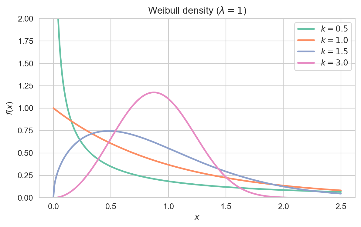
Interpretation: The shape \(k\) controls the hazard: \(k < 1\) gives a decreasing failure rate (early-life failures), \(k = 1\) a constant rate (the exponential case), and \(k > 1\) an increasing rate (wear-out).

Plotting code

import numpy as np
import matplotlib.pyplot as plt
import seaborn as sns
from scipy.stats import weibull_min

sns.set_style('whitegrid')
sns.set_palette('Set2')

x = np.linspace(0, 2.5, 400)
fig, ax = plt.subplots(figsize=(7, 4))
for k in (0.5, 1.0, 1.5, 3.0):
    ax.plot(x, weibull_min.pdf(x, k), lw=2, label=rf'$k = {k}$')

ax.set_xlabel('$x$')
ax.set_ylabel('$f(x)$')
ax.set_title(r'Weibull density ($\lambda = 1$)')
ax.set_ylim(0, 2)
ax.legend()
plt.show()

/Users/johnrobininston/Brain/Courses/PSTAT100/pstat100-2026-spring/.venv-pstat100-2026-spring/lib/python3.12/site-packages/scipy/stats/_continuous_distns.py:2760: RuntimeWarning: divide by zero encountered in power
  return c*pow(x, c-1)*np.exp(-pow(x, c))

Density of the Weibull distribution (\(\lambda = 1\)) for several shape parameters \(k\).

The cumulative distribution function is

\[ F(x) = 1 - \exp\!\left(-\left(\frac{x}{\lambda}\right)^k\right), \quad x \geq 0. \]

3 Key Properties

For \(X \sim \text{Weibull}(k, \lambda)\),

\[ \mathbb{E}[X] = \lambda\,\Gamma\!\left(1 + \frac{1}{k}\right), \]

\[ \operatorname{Var}(X) = \lambda^2 \left[\Gamma\!\left(1 + \frac{2}{k}\right) - \Gamma\!\left(1 + \frac{1}{k}\right)^2\right], \]

where \(\Gamma\) is the gamma function.

Proof. Substituting \(u = (x/\lambda)^k\) gives, for any \(n > 0\),

\[ \mathbb{E}[X^n] = \lambda^n \int_0^\infty u^{n/k} e^{-u} \, du = \lambda^n\,\Gamma\!\left(1 + \frac{n}{k}\right). \]

The mean and variance are the cases \(n = 1\) and \(n = 2\).

4 Relationship to Other Distributions

Exponential Distribution: \(\text{Weibull}(1, \lambda) = \text{Exponential}(1/\lambda)\).
Rayleigh Distribution: \(\text{Weibull}(2, \lambda)\) is a Rayleigh distribution with scale \(\lambda/\sqrt{2}\).
Gumbel Distribution: If \(X \sim \text{Weibull}(k, \lambda)\), then \(-\ln X\) follows a Gumbel distribution; both are extreme-value laws.

5 Examples and Applications

Component lifetimes with wear-out (\(k > 1\)) or infant-mortality (\(k < 1\)) failure modes are routinely modelled with a Weibull distribution.

The distribution of wind speeds at a site is commonly Weibull, which is used to estimate wind-power potential.

Time-to-event data with a monotone hazard — such as time to failure or time to recovery — are frequently fitted with Weibull models.

1 Introduction

2 Probability Density Function

3 Key Properties

4 Relationship to Other Distributions

5 Examples and Applications

6 Backlinks