The Maxwell-Boltzmann distribution is a continuous probability distribution for the speed of particles in an idealised gas at thermal equilibrium. It is the three-dimensional analogue of the Rayleigh Distribution: the magnitude of a vector with independent, zero-mean normal components.
A random variable \(X\) follows a Maxwell-Boltzmann distribution with scale parameter \(a > 0\) if
\[
X \sim \text{Maxwell}(a).
\]
2 Probability Density Function
The probability density function is
\[
f(x) = \sqrt{\frac{2}{\pi}}\,\frac{x^2}{a^3}
\exp\!\left(-\frac{x^2}{2a^2}\right),
\quad x \geq 0.
\]
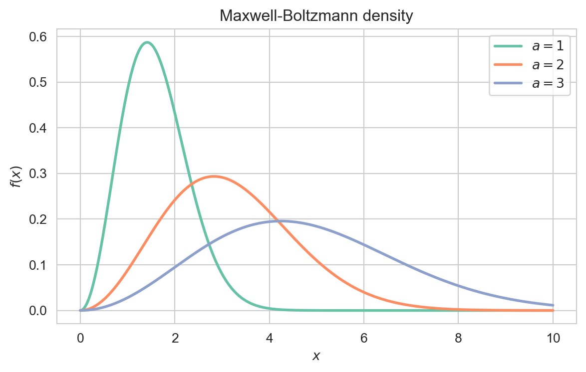
Interpretation: The factor \(x^2\) suppresses small speeds and the Gaussian factor suppresses large ones, giving a single peak at the most probable speed \(x = a\sqrt{2}\).
Plotting code
import numpy as npimport matplotlib.pyplot as pltimport seaborn as snsfrom scipy.stats import maxwellsns.set_style('whitegrid')sns.set_palette('Set2')x = np.linspace(0, 10, 400)fig, ax = plt.subplots(figsize=(7, 4))for a in (1, 2, 3): ax.plot(x, maxwell.pdf(x, scale=a), lw=2, label=rf'$a = {a}$')ax.set_xlabel('$x$')ax.set_ylabel('$f(x)$')ax.set_title('Maxwell-Boltzmann density')ax.legend()plt.show()
Density of the Maxwell-Boltzmann distribution for several scale parameters \(a\).