Dirichlet Distribution

1 Introduction

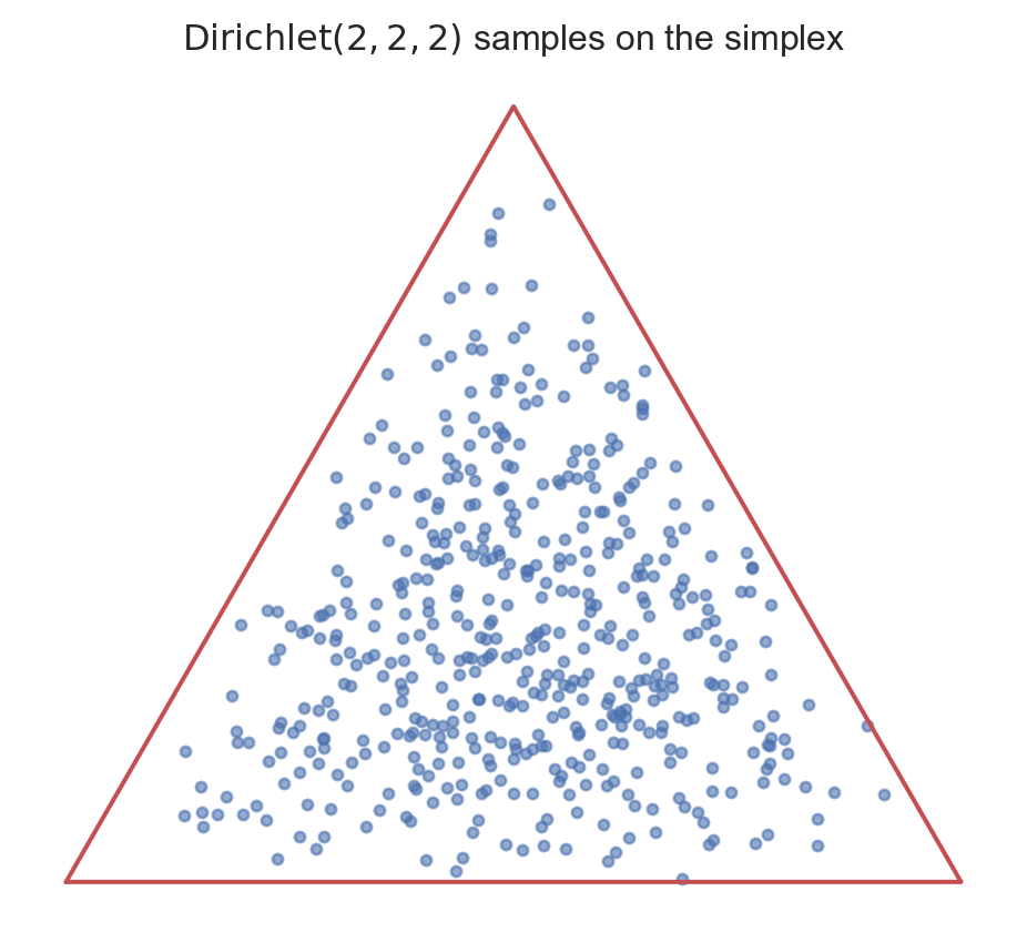
The Dirichlet distribution is a continuous multivariate probability distribution over the probability simplex — vectors of non-negative entries that sum to one. It is the multivariate generalisation of the Beta Distribution and the conjugate prior for the multinomial distribution.

A random vector \(\mathbf{X} = (X_1, \ldots, X_K)\) follows a Dirichlet distribution with concentration parameters \(\boldsymbol{\alpha} = (\alpha_1, \ldots, \alpha_K)\), each \(\alpha_i > 0\), if it is supported on the simplex \(\{\mathbf{x} : x_i \geq 0, \ \sum_i x_i = 1\}\) and

\[ \mathbf{X} \sim \text{Dirichlet}(\boldsymbol{\alpha}). \]

2 Probability Density Function

On the simplex the probability density function is

\[ f(\mathbf{x}) = \frac{1}{B(\boldsymbol{\alpha})} \prod_{i=1}^K x_i^{\alpha_i - 1}, \]

where the multivariate beta function is

\[ B(\boldsymbol{\alpha}) = \frac{\prod_{i=1}^K \Gamma(\alpha_i)} {\Gamma\!\left(\sum_{i=1}^K \alpha_i\right)}. \]

Interpretation: Writing \(\alpha_0 = \sum_i \alpha_i\), larger \(\alpha_0\) concentrates mass near the mean of the simplex, while values below one push mass toward the corners.

import numpy as np
import matplotlib.pyplot as plt
import seaborn as sns

sns.set_style('whitegrid')
sns.set_palette('Set2')

rng = np.random.default_rng(0)
samples = rng.dirichlet((2, 2, 2), size=500)

# Project barycentric coordinates onto a 2D equilateral triangle.
corners = np.array([[0, 0], [1, 0], [0.5, np.sqrt(3) / 2]])
pts = samples @ corners

fig, ax = plt.subplots(figsize=(6, 5.2))
triangle = np.vstack([corners, corners[0]])
ax.plot(triangle[:, 0], triangle[:, 1], color='#c44e52', lw=1.5)
ax.scatter(pts[:, 0], pts[:, 1], s=12, color='#4c72b0', alpha=0.6)

ax.set_title(r'$\text{Dirichlet}(2, 2, 2)$ samples on the simplex')
ax.set_aspect('equal')
ax.axis('off')
plt.show()

Samples from a \(\text{Dirichlet}(2, 2, 2)\) distribution, projected onto the 2-simplex (each point sums to one).

3 Key Properties

Let \(\alpha_0 = \sum_{i=1}^K \alpha_i\). For each component,

\[ \mathbb{E}[X_i] = \frac{\alpha_i}{\alpha_0}, \qquad \operatorname{Var}(X_i) = \frac{\alpha_i(\alpha_0 - \alpha_i)} {\alpha_0^2(\alpha_0 + 1)}, \]

and for \(i \neq j\) the components are negatively correlated,

\[ \operatorname{Cov}(X_i, X_j) = -\frac{\alpha_i \alpha_j} {\alpha_0^2(\alpha_0 + 1)}. \]

Proof. Each marginal \(X_i \sim \text{Beta}(\alpha_i, \alpha_0 - \alpha_i)\), from which the stated mean and variance follow directly. The covariance follows from the constraint \(\sum_i X_i = 1\), which forces the components to be negatively associated.

4 Relationship to Other Distributions

• Beta Distribution: For \(K = 2\), \(\text{Dirichlet}(\alpha_1, \alpha_2)\) reduces to \(\text{Beta}(\alpha_1, \alpha_2)\) on each marginal.
• Gamma Distribution: If \(Y_i \sim \text{Gamma}(\alpha_i, 1)\) are independent, then \((Y_1, \ldots, Y_K)/\sum_j Y_j \sim \text{Dirichlet}(\boldsymbol{\alpha})\).
• Multinomial: The Dirichlet is the conjugate prior for the category probabilities of a multinomial likelihood.

5 Examples and Applications

A Dirichlet prior on category probabilities, updated by multinomial counts, gives a Dirichlet posterior — the multivariate analogue of the Beta-Binomial model.

Latent Dirichlet Allocation places Dirichlet priors on document-topic and topic-word distributions to discover themes in text corpora.

Proportions that must sum to one — such as chemical compositions or market shares — are naturally modelled with the Dirichlet distribution.

6 Backlinks

• Beta Distribution
• Probability Distributions