Pareto Distribution

Author

John Robin Inston

Published

August 30, 2026

1 Introduction

The Pareto distribution is a continuous power-law probability distribution used to model quantities in which a small number of large values dominate — wealth, city sizes, and file sizes among them. It formalises the “80/20 rule”.

A random variable \(X\) follows a Pareto distribution with scale parameter \(x_m > 0\) (the minimum value) and shape parameter \(\alpha > 0\) if

\[ X \sim \text{Pareto}(x_m, \alpha). \]

2 Probability Density Function

The probability density function is

\[ f(x) = \frac{\alpha x_m^\alpha}{x^{\alpha + 1}}, \quad x \geq x_m. \]

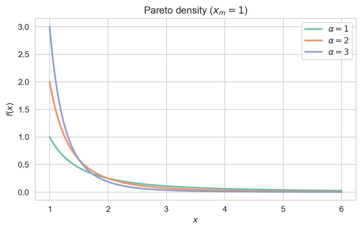
Interpretation: The density is largest at the lower bound \(x_m\) and decays as a power of \(x\), so large values are far more likely than under an exponentially decaying tail.

Plotting code
import numpy as np
import matplotlib.pyplot as plt
import seaborn as sns
from scipy.stats import pareto

sns.set_style('whitegrid')
sns.set_palette('Set2')

x = np.linspace(1, 6, 400)
fig, ax = plt.subplots(figsize=(7, 4))
for a in (1, 2, 3):
    ax.plot(x, pareto.pdf(x, a), lw=2, label=rf'$\alpha = {a}$')

ax.set_xlabel('$x$')
ax.set_ylabel('$f(x)$')
ax.set_title(r'Pareto density ($x_m = 1$)')
ax.legend()
plt.show()

Density of the Pareto distribution (\(x_m = 1\)) for several shape parameters \(\alpha\).
The cumulative distribution function is

\[ F(x) = 1 - \left(\frac{x_m}{x}\right)^\alpha, \quad x \geq x_m. \]

3 Key Properties

For \(X \sim \text{Pareto}(x_m, \alpha)\),

\[ \mathbb{E}[X] = \frac{\alpha x_m}{\alpha - 1} \ \ (\alpha > 1), \]

\[ \operatorname{Var}(X) = \frac{x_m^2 \alpha} {(\alpha - 1)^2 (\alpha - 2)} \ \ (\alpha > 2). \]

The mean is infinite for \(\alpha \leq 1\) and the variance is infinite for \(\alpha \leq 2\).

Proof. For \(\alpha > 1\),

\[ \mathbb{E}[X] = \int_{x_m}^\infty x \cdot \frac{\alpha x_m^\alpha}{x^{\alpha + 1}} \, dx = \alpha x_m^\alpha \int_{x_m}^\infty x^{-\alpha} \, dx = \frac{\alpha x_m}{\alpha - 1}. \]

The integral diverges when \(\alpha \leq 1\). The variance follows from the analogous computation of \(\mathbb{E}[X^2]\).

4 Relationship to Other Distributions

  • Exponential Distribution: If \(X \sim \text{Pareto}(x_m, \alpha)\), then \(\ln(X/x_m) \sim \text{Exponential}(\alpha)\).
  • Power law: The Pareto is the canonical continuous power-law distribution; the discrete analogue is the Zipf distribution.
  • Gumbel Distribution: Pareto tails place the distribution in the Fréchet domain of attraction for extreme values.

5 Examples and Applications

The upper tail of wealth and income distributions is well described by a Pareto law, the origin of the “80/20” observation.

City populations, firm sizes, file sizes on a server, and word frequencies all exhibit approximately Pareto-distributed tails.

Large claim sizes in insurance and operational losses are modelled with Pareto tails to capture the risk of rare, very large events.

6 Backlinks

Back to top