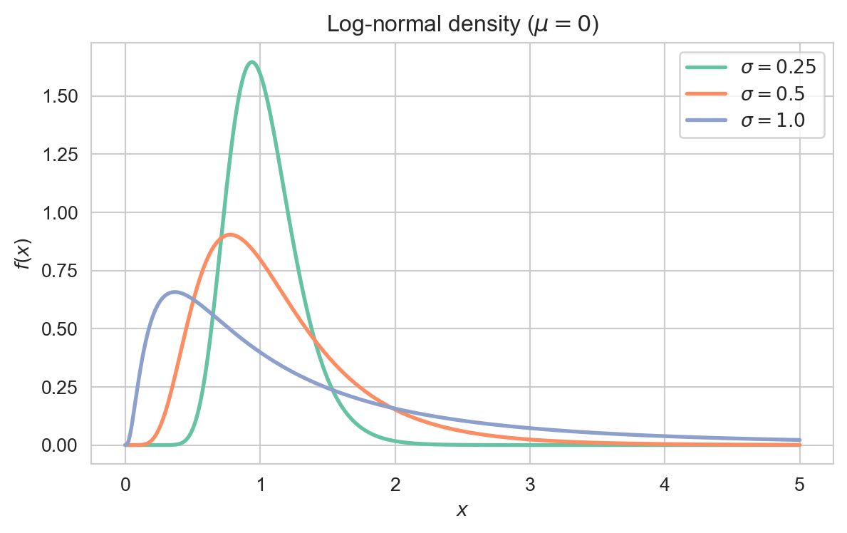
The log-normal distribution is a continuous probability distribution whose logarithm is normally distributed. It models positive-valued quantities that arise as the product of many independent positive factors.
A random variable \(X\) follows a log-normal distribution with parameters \(\mu \in \mathbb{R}\) and \(\sigma > 0\) if
\[
f(x) = \frac{1}{x\sigma\sqrt{2\pi}}
\exp\!\left(-\frac{(\ln x - \mu)^2}{2\sigma^2}\right),
\quad x > 0.
\]
Interpretation: The parameters \(\mu\) and \(\sigma\) are the mean and standard deviation of \(\ln(X)\), not of \(X\) itself. The density is right-skewed with a long upper tail.
Plotting code
import numpy as npimport matplotlib.pyplot as pltimport seaborn as snsfrom scipy.stats import lognormsns.set_style('whitegrid')sns.set_palette('Set2')x = np.linspace(0, 5, 400)fig, ax = plt.subplots(figsize=(7, 4))for sigma in (0.25, 0.5, 1.0): ax.plot(x, lognorm.pdf(x, sigma), lw=2, label=rf'$\sigma = {sigma}$')ax.set_xlabel('$x$')ax.set_ylabel('$f(x)$')ax.set_title(r'Log-normal density ($\mu = 0$)')ax.legend()plt.show()
Density of the log-normal distribution (\(\mu = 0\)) for several values of \(\sigma\).
The cumulative distribution function is
\[
F(x) = \Phi\!\left(\frac{\ln x - \mu}{\sigma}\right),
\quad x > 0,
\]
where \(\Phi\) is the CDF of the standard normal distribution.
3 Key Properties
The expectation and variance of \(X \sim \text{LogNormal}(\mu, \sigma^2)\) are
The stated mean and variance are the cases \(n = 1, 2\).
Note: Although all moments are finite, the moment generating function of \(X\) does not exist for any \(t > 0\), because the tail is too heavy.
4 Relationship to the Normal Distribution
If \(Y \sim \mathcal{N}(\mu, \sigma^2)\) then \(X = e^Y \sim
\text{LogNormal}(\mu, \sigma^2)\), and conversely \(\ln(X) \sim
\mathcal{N}(\mu, \sigma^2)\). This exponential link, together with a multiplicative Central Limit Theorem, makes the log-normal the natural limit of products of independent positive factors.
The distribution is right-skewed, and its median lies below its mean:
Normal Distribution:\(\ln(X)\) is normal; the log-normal is its exponential image.
Geometric Brownian motion: The value of a Random Variable Transformations of Brownian motion at a fixed time is log-normally distributed, underpinning models of asset prices.
6 Applications and Examples
Stock prices and asset returns are often modelled as log-normal, as in geometric Brownian motion.