Classification

An introduction to classification including logistic regression for multiple classes, decision trees with Gini impurity and pruning, and random forests as a variance-reducing ensemble method.

ImportantLearning Objectives

• Understand the classification problem and how it differs from regression.
• Extend logistic regression to multiple classes using the softmax (multinomial) formulation.
• Define Gini impurity and describe how decision trees are grown using recursive binary splitting.
• Control overfitting with pre-pruning parameters and cost-complexity post-pruning.
• Describe random forests as bagging with feature subsampling, and interpret mean decrease in impurity.
• Evaluate classifiers with confusion matrices, precision, recall, and F1-score.

import numpy as np
import pandas as pd
import matplotlib.pyplot as plt
import seaborn as sns
from matplotlib.colors import ListedColormap

from sklearn.linear_model import LogisticRegression
from sklearn.tree import DecisionTreeClassifier, plot_tree
from sklearn.ensemble import RandomForestClassifier
from sklearn.preprocessing import StandardScaler, LabelEncoder
from sklearn.impute import SimpleImputer
from sklearn.model_selection import train_test_split
from sklearn.metrics import (
    confusion_matrix, ConfusionMatrixDisplay,
    classification_report, accuracy_score,
    precision_recall_fscore_support,
)
from sklearn.datasets import make_circles

sns.set_style('whitegrid')
sns.set_palette('Set2')

From Regression to Classification

In regression, the response is continuous: \(Y \in \mathbb{R}\). In classification, the response is categorical: \(Y \in \{1, 2, \ldots, K\}\). The goal is to learn a decision rule \(\hat{f}: \mathcal{X} \to \{1, \ldots, K\}\) that maps features to class labels as accurately as possible.

Task	Response classes
Email spam detection	Spam / Not Spam
Medical diagnosis	Disease / No Disease
Handwritten digit recognition	0, 1, 2, …, 9
Species identification	Species A, B, C, …

Logistic Regression for Multiple Classes

Binary logistic regression (covered in the GLM chapter) models the probability of the positive class via the sigmoid function. For \(K > 2\) classes, there are two standard extensions.

One-vs-Rest (OvR): fit \(K\) separate binary classifiers, each asking “is this class \(k\) or not?”. Predict the class whose classifier returns the highest probability.

Multinomial (softmax): fit all classes simultaneously:

\[P(Y = k \mid \mathbf{x}) = \frac{\exp(\mathbf{x}^\top \boldsymbol{\beta}_k)}{\displaystyle\sum_{j=1}^{K} \exp(\mathbf{x}^\top \boldsymbol{\beta}_j)}.\]

sklearn’s LogisticRegression uses the multinomial approach by default for \(K > 2\). The decision boundary remains linear — each class is still separated by a hyperplane.

Why go beyond logistic regression?

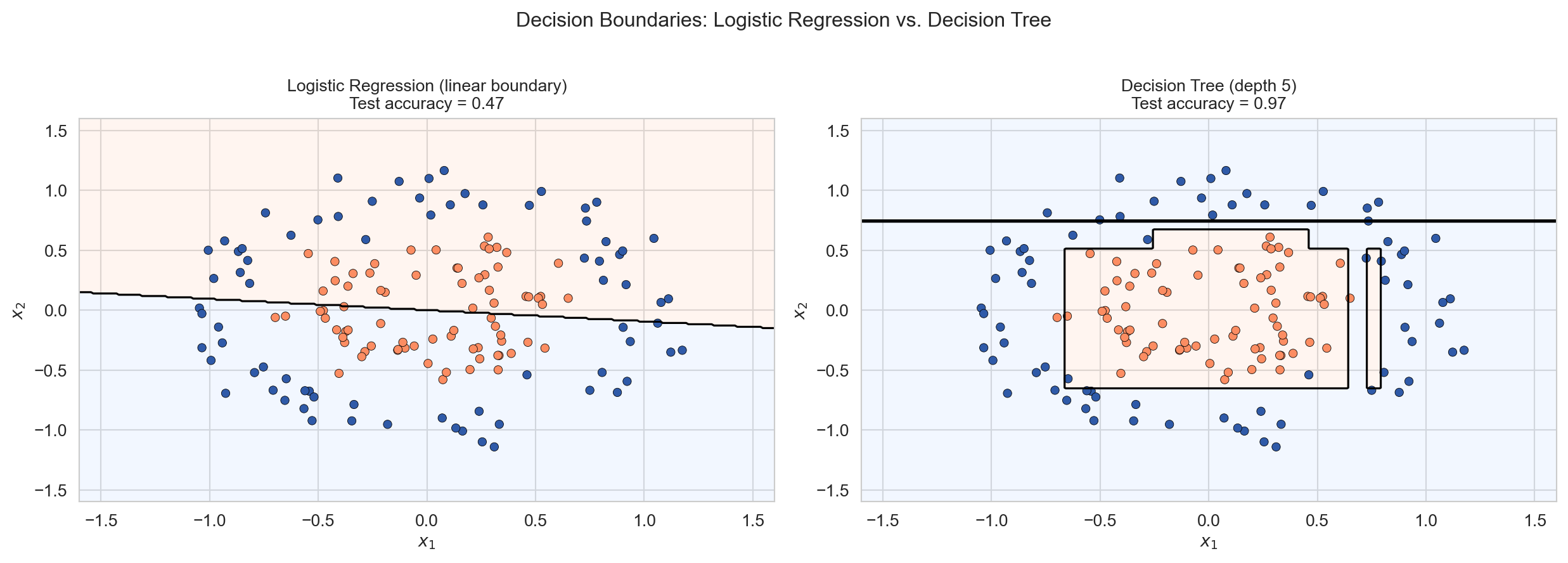
When the true decision boundary is non-linear, logistic regression is structurally unable to recover it regardless of sample size.

Two concentric circles cannot be separated by any straight line — logistic regression fails. A decision tree carves the space into axis-aligned rectangles and recovers the circular boundary well.

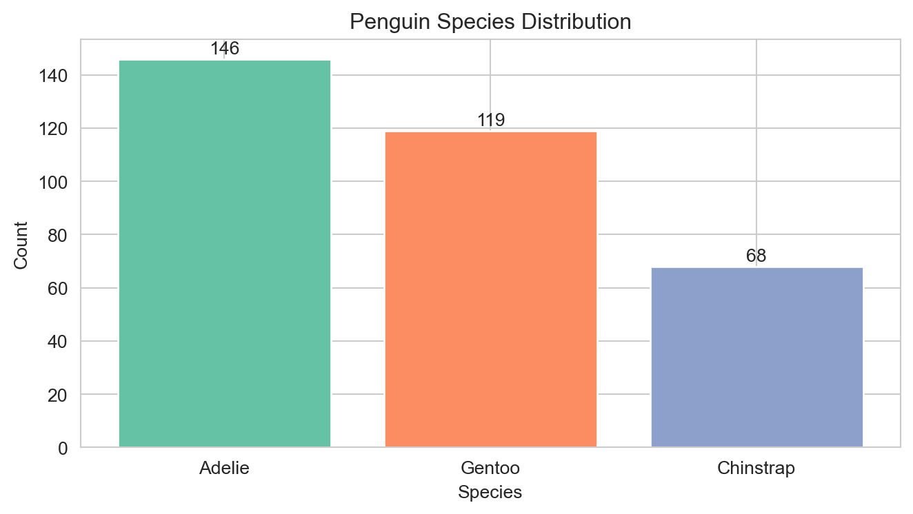
The Palmer Penguins Dataset

We use the Palmer Penguins dataset — a multiclass classification benchmark with three penguin species measured across physical characteristics.

• Response: species — Adelie, Chinstrap, Gentoo (three classes).
• Predictors: bill length, bill depth, flipper length, body mass, sex, island.
• \(n = 344\) penguins with some missing values.

penguins = sns.load_dataset('penguins').dropna()
print(penguins.shape)
penguins.head()

(333, 7)

	species	island	bill_length_mm	bill_depth_mm	flipper_length_mm	body_mass_g	sex
0	Adelie	Torgersen	39.1	18.7	181.0	3750.0	Male
1	Adelie	Torgersen	39.5	17.4	186.0	3800.0	Female
2	Adelie	Torgersen	40.3	18.0	195.0	3250.0	Female
4	Adelie	Torgersen	36.7	19.3	193.0	3450.0	Female
5	Adelie	Torgersen	39.3	20.6	190.0	3650.0	Male

fig, ax = plt.subplots(figsize=(7, 4))
counts = penguins['species'].value_counts()
ax.bar(counts.index, counts.values, color=sns.color_palette('Set2', 3), edgecolor='white')
for i, (sp, cnt) in enumerate(counts.items()):
    ax.text(i, cnt + 2, f'{cnt}', ha='center', fontsize=10)
ax.set_xlabel('Species'); ax.set_ylabel('Count')
ax.set_title('Penguin Species Distribution')
plt.tight_layout()
plt.show()

Class distribution of the three penguin species. Adelie is the largest class; Chinstrap the smallest — mild imbalance that matters for evaluation.

Preprocessing and train-test split

We encode the categorical target and predictors, then split 80/20 with stratification to preserve class proportions.

# Encode target
le = LabelEncoder()
y  = le.fit_transform(penguins['species'])   # 0=Adelie, 1=Chinstrap, 2=Gentoo

# Encode categorical features and standardise numeric ones
X_num = penguins[['bill_length_mm', 'bill_depth_mm',
                   'flipper_length_mm', 'body_mass_g']].values
X_cat = pd.get_dummies(penguins[['island', 'sex']], drop_first=True).values.astype(float)
X     = np.hstack([X_num, X_cat])

scaler = StandardScaler()
X_num_s = scaler.fit_transform(X_num)
X_proc  = np.hstack([X_num_s, X_cat])

X_train, X_test, y_train, y_test = train_test_split(
    X_proc, y, test_size=0.2, stratify=y, random_state=42
)
feature_names = ['bill_length', 'bill_depth', 'flipper_length', 'body_mass',
                 'island_Dream', 'island_Torgersen', 'sex_male']
print(f"Train: {X_train.shape[0]}   Test: {X_test.shape[0]}")

Train: 266   Test: 67

Evaluating Classifiers

Before fitting models it helps to understand the evaluation metrics we will use.

Accuracy is the simplest: fraction of all predictions that are correct. But accuracy can be misleading when classes are imbalanced — a classifier predicting only the majority class can still achieve high accuracy.

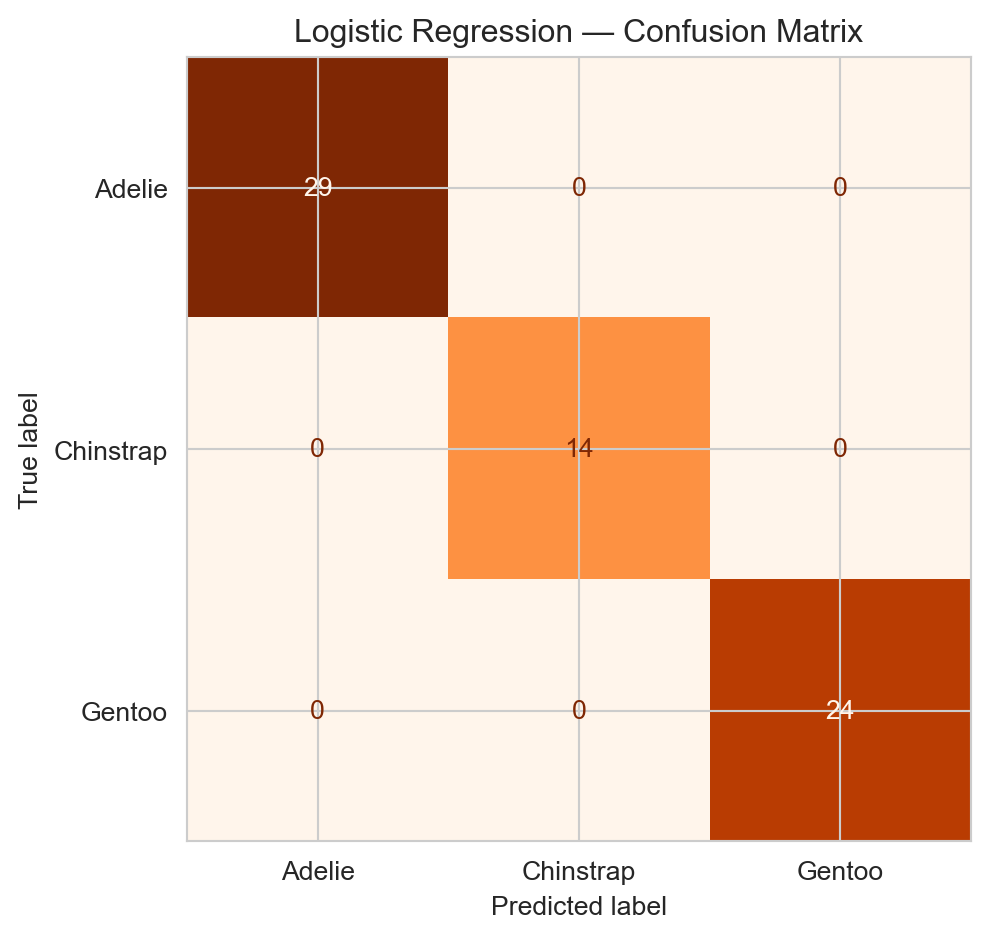
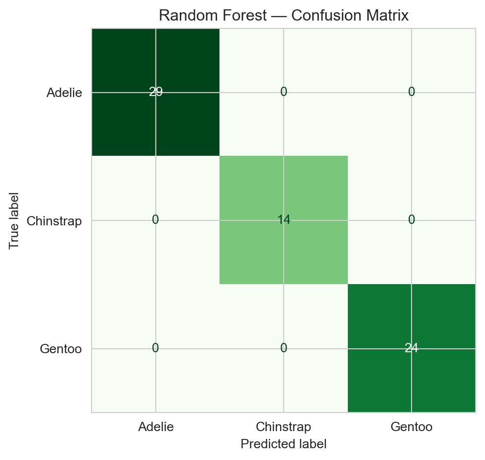
ImportantConfusion Matrix

For \(K\) classes, a \(K \times K\) table where entry \((i, j)\) is the number of observations of true class \(i\) predicted as class \(j\). Diagonal entries are correct predictions; off-diagonal entries are misclassifications.

For each class \(k\), treating it as “positive” vs. all others:

\[\text{Precision}_k = \frac{TP_k}{TP_k + FP_k} \qquad \text{Recall}_k = \frac{TP_k}{TP_k + FN_k} \qquad F_{1,k} = \frac{2 \cdot \text{Pr}_k \cdot \text{Re}_k}{\text{Pr}_k + \text{Re}_k}\]

• Precision: of all observations predicted as class \(k\), what fraction truly belong to \(k\)?
• Recall: of all observations that truly belong to class \(k\), what fraction were correctly identified?
• F1: harmonic mean of precision and recall — useful when both matter equally.

Logistic Regression in Practice

lr = LogisticRegression(max_iter=1000, random_state=42)
lr.fit(X_train, y_train)
y_pred_lr = lr.predict(X_test)
print(f"Validation accuracy: {accuracy_score(y_test, y_pred_lr):.4f}\n")
print(classification_report(y_test, y_pred_lr, target_names=le.classes_))

Validation accuracy: 1.0000

              precision    recall  f1-score   support

      Adelie       1.00      1.00      1.00        29
   Chinstrap       1.00      1.00      1.00        14
      Gentoo       1.00      1.00      1.00        24

    accuracy                           1.00        67
   macro avg       1.00      1.00      1.00        67
weighted avg       1.00      1.00      1.00        67

fig, ax = plt.subplots(figsize=(6, 5))
ConfusionMatrixDisplay(
    confusion_matrix(y_test, y_pred_lr),
    display_labels=le.classes_,
).plot(ax=ax, colorbar=False, cmap='Oranges')
ax.set_title('Logistic Regression — Confusion Matrix')
plt.tight_layout()
plt.show()

Confusion matrix for logistic regression on the test set.

Decision Trees

What is a decision tree?

A decision tree partitions the feature space into rectangular regions using a recursive sequence of binary splits. Each leaf is assigned the majority class of training observations that land there. Decision trees are fully non-parametric — no distributional assumption about the boundary shape.

Gini impurity

At each node we search for the feature \(j\) and threshold \(t\) that most reduce impurity in the resulting child nodes.

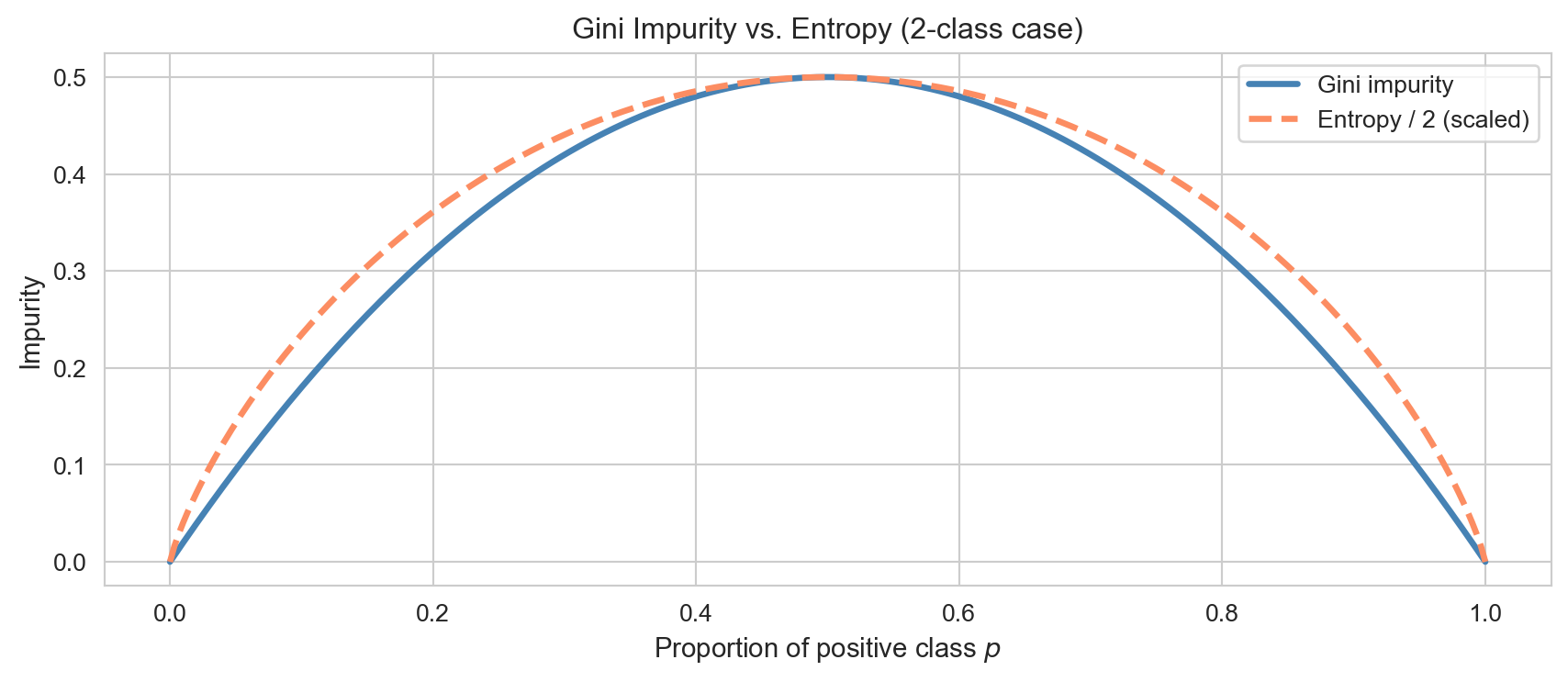
ImportantGini Impurity

For a node containing observations with class proportions \(p_1, \ldots, p_K\): \[G = 1 - \sum_{k=1}^{K} p_k^2.\] \(G = 0\) means the node is pure (all one class). \(G\) is maximised when classes are equally represented.

The Gini gain of a candidate split is: \[\Delta G = G(\text{parent}) - \frac{n_L}{n}\,G(\text{left}) - \frac{n_R}{n}\,G(\text{right}).\] The best split \((j^*, t^*)\) maximises \(\Delta G\).

Gini impurity and entropy as functions of the positive-class proportion in a 2-class problem. Both are maximised at p = 0.5 and zero at pure nodes.

Growing and stopping a tree

A tree is grown recursively: find the best split, partition observations into left and right children, and recurse. Key stopping parameters in sklearn are:

Parameter	Effect
max_depth	Hard cap on tree height
min_samples_split	Minimum observations needed to attempt a split
min_samples_leaf	Minimum observations required in each leaf
min_impurity_decrease	Only split if \(\Delta G\) exceeds this threshold

Overfitting

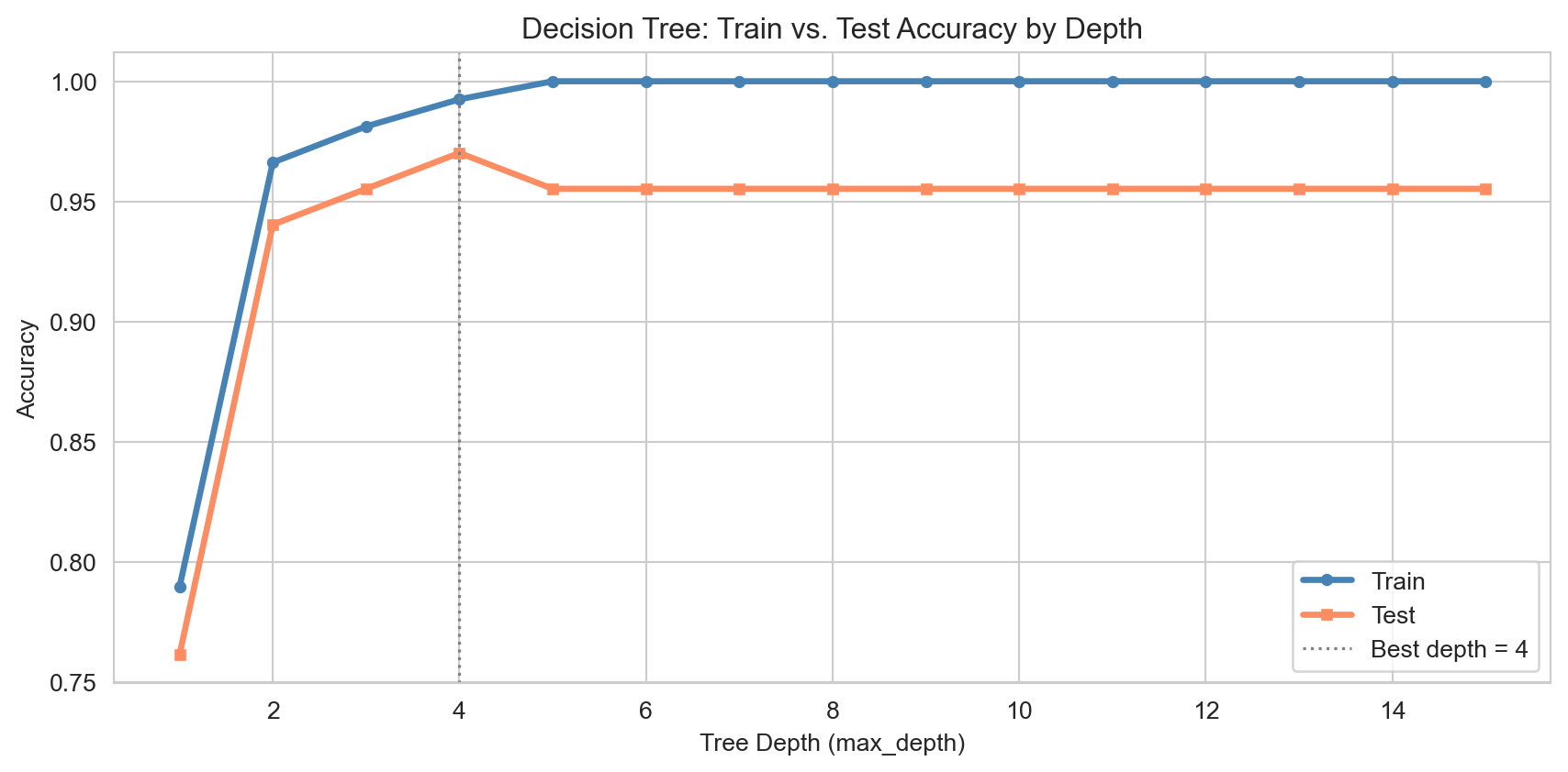
Deep trees memorise the training set rather than learning general patterns.

depths     = range(1, 16)
train_accs = []
test_accs  = []

for d in depths:
    clf = DecisionTreeClassifier(max_depth=d, random_state=42)
    clf.fit(X_train, y_train)
    train_accs.append(accuracy_score(y_train, clf.predict(X_train)))
    test_accs.append(accuracy_score(y_test, clf.predict(X_test)))

fig, ax = plt.subplots(figsize=(9, 4.5))
ax.plot(depths, train_accs, lw=2.5, color='steelblue', marker='o', ms=4, label='Train')
ax.plot(depths, test_accs,  lw=2.5, color='#fc8d62',   marker='s', ms=4, label='Test')
best_d = int(np.argmax(test_accs)) + 1
ax.axvline(best_d, color='gray', lw=1.2, linestyle=':', label=f'Best depth = {best_d}')
ax.set_xlabel('Tree Depth (max_depth)'); ax.set_ylabel('Accuracy')
ax.set_title('Decision Tree: Train vs. Test Accuracy by Depth')
ax.legend(fontsize=10)
plt.tight_layout()
plt.show()

Train and test accuracy by tree depth. Shallow trees underfit; very deep trees overfit.

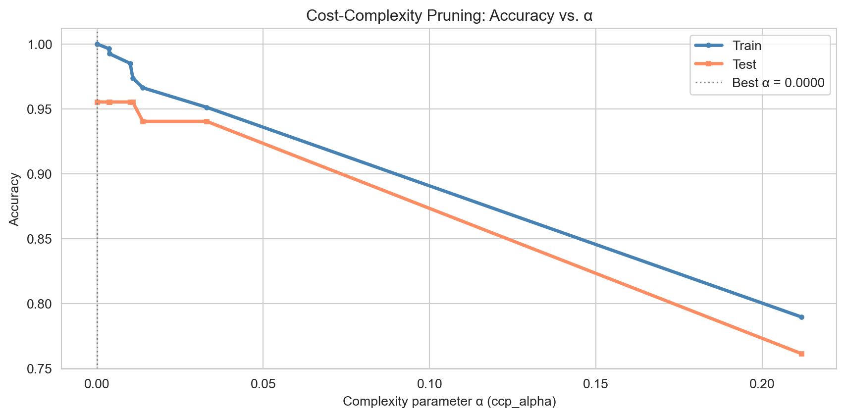
Post-pruning: cost-complexity

Pre-pruning uses stopping criteria to prevent the tree from growing too large. Post-pruning takes the opposite approach: grow the full tree, then cut back branches whose impurity reduction is outweighed by their complexity cost.

ImportantCost-Complexity Criterion

For a subtree \(T\) with \(|T|\) leaves, define the penalised training cost: \[R_\alpha(T) = R(T) + \alpha \cdot |T|,\] where \(R(T)\) is the weighted leaf impurity and \(\alpha \geq 0\) is the complexity parameter.

At \(\alpha = 0\) the full unpruned tree is returned. As \(\alpha\) increases, branches are progressively removed. The optimal \(\alpha\) is chosen by evaluating held-out performance across the pruning path.

path   = DecisionTreeClassifier(random_state=42).cost_complexity_pruning_path(X_train, y_train)
alphas = path.ccp_alphas[:-1]
step   = max(1, len(alphas) // 40)
alphas = alphas[::step]

train_p, test_p = [], []
for a in alphas:
    clf = DecisionTreeClassifier(ccp_alpha=a, random_state=42)
    clf.fit(X_train, y_train)
    train_p.append(accuracy_score(y_train, clf.predict(X_train)))
    test_p.append(accuracy_score(y_test, clf.predict(X_test)))

best_alpha = alphas[int(np.argmax(test_p))]
fig, ax = plt.subplots(figsize=(9, 4.5))
ax.plot(alphas, train_p, lw=2.5, color='steelblue', marker='o', ms=3, label='Train')
ax.plot(alphas, test_p,  lw=2.5, color='#fc8d62',   marker='s', ms=3, label='Test')
ax.axvline(best_alpha, color='gray', lw=1.2, linestyle=':', label=f'Best α = {best_alpha:.4f}')
ax.set_xlabel('Complexity parameter α (ccp_alpha)'); ax.set_ylabel('Accuracy')
ax.set_title('Cost-Complexity Pruning: Accuracy vs. α')
ax.legend(fontsize=10)
plt.tight_layout()
plt.show()

Validation accuracy peaks at an intermediate α — just enough pruning to improve generalisation without discarding useful splits.

Fitting and visualising the decision tree

dt = DecisionTreeClassifier(max_depth=best_d, min_samples_leaf=5, random_state=42)
dt.fit(X_train, y_train)
y_pred_dt = dt.predict(X_test)
print(f"Test accuracy: {accuracy_score(y_test, y_pred_dt):.4f}\n")
print(classification_report(y_test, y_pred_dt, target_names=le.classes_))

Test accuracy: 0.9403

              precision    recall  f1-score   support

      Adelie       0.97      0.97      0.97        29
   Chinstrap       0.81      0.93      0.87        14
      Gentoo       1.00      0.92      0.96        24

    accuracy                           0.94        67
   macro avg       0.93      0.94      0.93        67
weighted avg       0.95      0.94      0.94        67

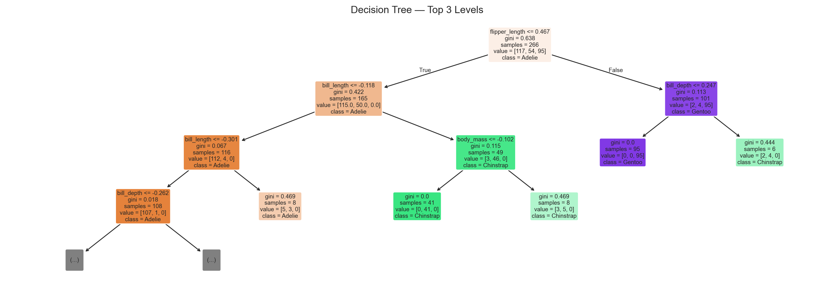
fig, ax = plt.subplots(figsize=(14, 5))
plot_tree(
    dt, max_depth=3, feature_names=feature_names,
    class_names=le.classes_, filled=True, rounded=True, fontsize=7, ax=ax,
)
ax.set_title('Decision Tree — Top 3 Levels')
plt.tight_layout()
plt.show()

Top 3 levels of the fitted decision tree. Each node shows the splitting feature, Gini impurity, sample count, and class distribution. Leaf colours indicate the predicted class.

fig, ax = plt.subplots(figsize=(6, 5))
ConfusionMatrixDisplay(
    confusion_matrix(y_test, y_pred_dt), display_labels=le.classes_,
).plot(ax=ax, colorbar=False, cmap='Blues')
ax.set_title('Decision Tree — Confusion Matrix')
plt.tight_layout()
plt.show()

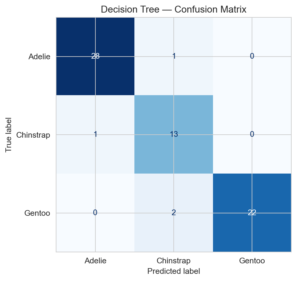
Confusion matrix for the decision tree on the test set.

Random Forests

The variance problem with single trees

Decision trees have high variance: small changes in the training data can produce very different trees. Each split depends entirely on which observations happened to be in the training set; a single influential observation can redirect an entire branch.

Bagging: Bootstrap Aggregating

ImportantBagging Algorithm

For \(b = 1, \ldots, B\):

1. Draw a bootstrap sample \(\mathcal{D}^*_b\) of size \(n\) with replacement.
2. Fit a full, unpruned tree \(T_b\) on \(\mathcal{D}^*_b\).

Prediction: \(\hat{y} = \text{mode}\!\left\{T_1(\mathbf{x}), \ldots, T_B(\mathbf{x})\right\}\).

Each tree sees \(\approx 63\%\) of observations; the rest form a natural out-of-bag (OOB) validation set. Averaging over \(B\) trees reduces variance — provided trees are uncorrelated.

Feature subsampling: the random forest improvement

If one feature is very strong, all bagged trees split on it first — the trees are correlated and the variance reduction is limited.

ImportantRandom Forest

Bagging + feature subsampling: at each candidate split, consider only a random subset of \(m\) features (default: \(m = \lfloor\sqrt{p}\rfloor\)) rather than all \(p\).

Restricting the features considered per split decorrelates the trees, giving greater variance reduction. The slight bias increase from seeing fewer features per split is usually outweighed by the variance benefit.

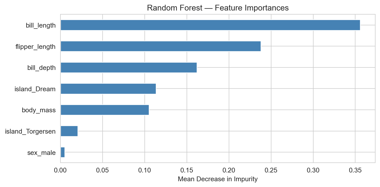
Feature importance: Mean Decrease in Impurity

ImportantMean Decrease in Impurity (MDI)

For feature \(j\), sum the weighted Gini gain from every split on \(j\) across all trees: \[\text{Importance}(j) = \frac{1}{B}\sum_{b=1}^{B} \sum_{\substack{v \in T_b \\ \text{split on } j}} \frac{n_v}{n}\,\Delta G_v.\]

ImportantCaveat

MDI can overstate importance for high-cardinality or continuous features. Permutation importance is a more reliable alternative in such cases.

Fitting a random forest

rf = RandomForestClassifier(
    n_estimators=200,
    max_features='sqrt',
    min_samples_leaf=3,
    oob_score=True,
    n_jobs=-1,
    random_state=42,
)
rf.fit(X_train, y_train)
y_pred_rf = rf.predict(X_test)

print(f"OOB accuracy:  {rf.oob_score_:.4f}")
print(f"Test accuracy: {accuracy_score(y_test, y_pred_rf):.4f}\n")
print(classification_report(y_test, y_pred_rf, target_names=le.classes_))

OOB accuracy:  0.9887
Test accuracy: 1.0000

              precision    recall  f1-score   support

      Adelie       1.00      1.00      1.00        29
   Chinstrap       1.00      1.00      1.00        14
      Gentoo       1.00      1.00      1.00        24

    accuracy                           1.00        67
   macro avg       1.00      1.00      1.00        67
weighted avg       1.00      1.00      1.00        67

fig, ax = plt.subplots(figsize=(6, 5))
ConfusionMatrixDisplay(
    confusion_matrix(y_test, y_pred_rf), display_labels=le.classes_,
).plot(ax=ax, colorbar=False, cmap='Greens')
ax.set_title('Random Forest — Confusion Matrix')
plt.tight_layout()
plt.show()

Confusion matrix for the random forest on the test set.

importances = pd.Series(rf.feature_importances_, index=feature_names).sort_values()
fig, ax = plt.subplots(figsize=(8, 4))
importances.plot.barh(ax=ax, color='steelblue', edgecolor='white')
ax.set_xlabel('Mean Decrease in Impurity')
ax.set_title('Random Forest — Feature Importances')
plt.tight_layout()
plt.show()

Feature importances by mean decrease in Gini impurity. Flipper length and bill length are the most discriminative features across the three penguin species.

Comparing All Three Classifiers

classes = le.classes_.tolist()
results = {}
for name, pred in [('Logistic Reg.', y_pred_lr),
                   ('Decision Tree', y_pred_dt),
                   ('Random Forest', y_pred_rf)]:
    p, r, f, _ = precision_recall_fscore_support(y_test, pred, labels=[0, 1, 2])
    results[name] = pd.DataFrame({'Class': classes, 'Precision': p, 'Recall': r, 'F1': f})

combined = (
    pd.concat(results, names=['Model'])
    .reset_index(level=0)
    .rename(columns={'level_0': 'Model'})
)
melted = combined.melt(id_vars=['Model', 'Class'],
                       value_vars=['Precision', 'Recall', 'F1'],
                       var_name='Metric', value_name='Score')

fig, axes = plt.subplots(1, 3, figsize=(13, 4.5), sharey=True)
palette = ['#fc8d62', 'steelblue', '#66c2a5']
for ax, metric in zip(axes, ['Precision', 'Recall', 'F1']):
    sub = melted[melted['Metric'] == metric]
    sns.barplot(data=sub, x='Class', y='Score', hue='Model', ax=ax, palette=palette)
    ax.set_title(metric, fontsize=11); ax.set_ylim(0, 1.05)
    ax.set_xlabel(''); ax.set_ylabel('Score' if ax is axes[0] else '')
    ax.legend(fontsize=7)

plt.suptitle('Logistic Regression vs. Decision Tree vs. Random Forest — Per-Class Metrics',
             fontsize=11, y=1.02)
plt.tight_layout()
plt.show()

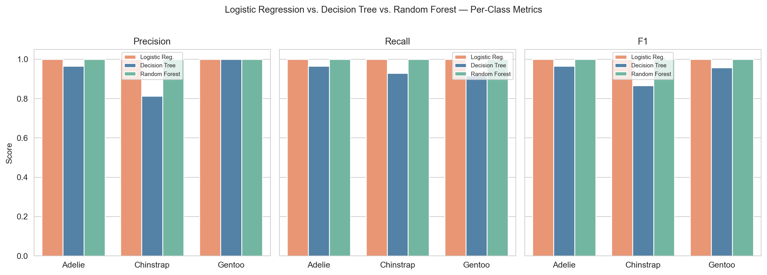
Per-class precision, recall, and F1 for all three classifiers. The random forest leads across most metrics; logistic regression sets the linear baseline.

summary = pd.DataFrame({
    'Model':              ['Logistic Regression', 'Decision Tree', 'Random Forest (200 trees)'],
    'Test Accuracy':      [round(accuracy_score(y_test, y_pred_lr), 4),
                           round(accuracy_score(y_test, y_pred_dt), 4),
                           round(accuracy_score(y_test, y_pred_rf), 4)],
    'OOB Accuracy':       ['—', '—', round(rf.oob_score_, 4)],
    'Linear boundary?':   ['Yes', 'No', 'No'],
    'Interpretable?':     ['Coefficients', 'Tree diagram', 'Feature importance only'],
})
print(summary.to_string(index=False))

                    Model  Test Accuracy OOB Accuracy Linear boundary?          Interpretable?
      Logistic Regression         1.0000            —              Yes            Coefficients
            Decision Tree         0.9403            —               No            Tree diagram
Random Forest (200 trees)         1.0000       0.9887               No Feature importance only