Data Preparation

Data preparation in python including missingness, duplicates, fixing data types, relabeling, and more.

Author

John Robin Inston

Published

May 6, 2026

Modified

May 22, 2026

Learning Objectives

Understand what data preparation is and why it is necessary.
Diagnose and handle missing data, including the MCAR / MAR / MNAR classification.
Identify and remove or aggregate duplicate records.
Fix inconsistent and mixed data types, including dates and booleans.
Detect and resolve invalid values and labelling inconsistencies.
Follow a principled, step-by-step data preparation workflow.

Libraries

import pandas as pd
import numpy as np
import missingno as msno
import matplotlib.pyplot as plt
import seaborn as sns

sns.set_style('whitegrid')
sns.set_palette('Set2')

Tidy Data and Common Problems

In the previous chapter we introduced the tidy data standard:

Tidy Data Standard

For data to be tidy it must satisfy the following three rules:

Each variable is a column.
Each observation is a row.
Each type of observational unit forms a table.

In practice, raw data almost never arrives in this form. Beyond structure, real datasets routinely contain:

Missing values — entries that were never collected, lost, or recorded incorrectly.
Duplicate records — rows that represent the same observation more than once.
Inconsistent or incorrect data types — dates stored as strings, numbers encoded as text.
Invalid values — entries that appear real but break domain rules (e.g. a negative age).
Labelling issues — the same category written in multiple ways across rows or files.

Data preparation is the process of systematically identifying and resolving these problems before analysis.

Data Preparation

Data preparation is the process of cleaning and transforming data to make it suitable for analysis.

The workflow for each problem follows the same pattern:

Identify — find what is wrong with the data.
Determine — decide how to fix the problem.
Update and check — apply the fix and verify the result.

Missing Data

Causes and consequences

Missing data can arise for many reasons: a field was never collected, data was collected but subsequently lost, or a value was recorded incorrectly and then nullified. Understanding why data is missing is important because it determines what treatment is appropriate.

Classifying missingness

There are three standard classifications:

Missing Completely at Random (MCAR) — missingness is independent of both observed and unobserved data. Deleting missing rows introduces no bias.
Missing at Random (MAR) — missingness can be fully accounted for by other observed variables. Imputation using those variables is justified.
Missing Not at Random (MNAR) — missingness depends on the missing value itself or on unobserved factors. This is the most problematic case and requires careful modelling.

Missingness is often informative in its own right. A blank income field may mean the respondent preferred not to disclose it (biasing a sample toward lower earners). Missing follow-up appointments in a clinical trial may indicate patients who became too ill to return (biasing an efficacy estimate upward). Ignoring these patterns leads to biased analysis.

Practice data

We will use a synthetic student academic records dataset throughout this section. It has enough columns and varied missingness patterns to illustrate the key tools.

Creating synthetic student dataset with missing values.

rng = np.random.default_rng(42)
n = 500

year  = rng.choice([1, 2, 3, 4], size=n, p=[0.25, 0.25, 0.25, 0.25])
gpa   = rng.normal(3.0, 0.5, size=n).clip(0, 4.0)

# SAT score — missing for ~15% (some students sat the ACT instead)
sat = rng.integers(900, 1600, size=n).astype(float)
sat[rng.random(n) < 0.15] = np.nan

# Income bracket and parent education — sensitive fields, often missing together
income_mask   = rng.random(n) < 0.30
parent_mask   = income_mask | (rng.random(n) < 0.10)
income        = pd.Series(rng.choice(["Low", "Middle", "High"], size=n), dtype=object)
parent_ed     = pd.Series(rng.choice(["High School", "Some College", "Bachelor's", "Graduate"], size=n), dtype=object)
income[income_mask]     = np.nan
parent_ed[parent_mask]  = np.nan

study_hours   = rng.integers(5, 40, size=n).astype(float)
study_hours[rng.random(n) < 0.10] = np.nan

internship    = rng.choice([0, 1], size=n).astype(float)
internship[rng.random(n) < 0.25] = np.nan

# Research hours — mostly missing for first- and second-year students
research      = rng.integers(0, 20, size=n).astype(float)
research[(year < 3) | (rng.random(n) < 0.30)] = np.nan

# Scholarship and financial aid — correlated missingness
scholarship_mask  = rng.random(n) < 0.20
scholarship       = rng.choice([0, 1], size=n).astype(float)
financial_aid     = rng.integers(0, 20000, size=n).astype(float)
scholarship[scholarship_mask] = np.nan
financial_aid[scholarship_mask | (rng.random(n) < 0.10)] = np.nan

# Thesis score — only exists for year-4 students
thesis = rng.normal(75, 10, size=n).clip(0, 100)
thesis[year < 4] = np.nan

mentor         = rng.choice([0, 1], size=n).astype(float)
mentor[rng.random(n) < 0.05] = np.nan

# Exit survey — only year-4 students, and only ~40% completed it
exit_survey = rng.integers(1, 10, size=n).astype(float)
exit_survey[(year < 4) | (rng.random(n) < 0.60)] = np.nan

students = pd.DataFrame({
    'student_id':    [f"S{str(i).zfill(4)}" for i in range(1, n + 1)],
    'year':          year,
    'gpa':           gpa,
    'sat_score':     sat,
    'income_bracket': income,
    'parent_education': parent_ed,
    'study_hours_wk': study_hours,
    'internship':    internship,
    'research_hours': research,
    'scholarship':   scholarship,
    'financial_aid': financial_aid,
    'thesis_score':  thesis,
    'mentor_assigned': mentor,
    'exit_survey_score': exit_survey,
})

Inspecting missingness

The first step is to understand the scale of the problem.

students.head()

	student_id	year	gpa	sat_score	income_bracket	parent_education	study_hours_wk	internship	research_hours	scholarship	financial_aid	thesis_score	mentor_assigned	exit_survey_score
0	S0001	4	3.716607	1267.0	NaN	NaN	34.0	0.0	NaN	NaN	NaN	67.096113	1.0	8.0
1	S0002	2	3.045760	1139.0	NaN	NaN	16.0	1.0	NaN	0.0	9065.0	NaN	1.0	NaN
2	S0003	4	3.290389	1289.0	Middle	Graduate	7.0	0.0	13.0	NaN	NaN	74.403315	1.0	8.0
3	S0004	3	2.971608	1024.0	NaN	NaN	12.0	1.0	5.0	NaN	NaN	NaN	1.0	NaN
4	S0005	1	2.914796	963.0	NaN	NaN	22.0	1.0	NaN	NaN	NaN	NaN	1.0	NaN

students.shape

(500, 14)

We count missing values per column and compute an overall percentage.

missing_counts = students.isnull().sum().sort_values(ascending=False)
missing_counts

exit_survey_score    443
thesis_score         376
research_hours       322
parent_education     195
income_bracket       155
financial_aid        143
internship           135
scholarship          105
sat_score             61
study_hours_wk        49
mentor_assigned       18
student_id             0
year                   0
gpa                    0
dtype: int64

total_cells   = np.prod(students.shape)
total_missing = missing_counts.sum()
print(f"Overall missingness: {total_missing / total_cells * 100:.1f}%")

Overall missingness: 28.6%

Visualising missingness with `missingno`

The missingno library provides four complementary views of missing data patterns.

Bar chart — shows the count of non-null values per column at a glance.

msno.bar(students, figsize=(9, 5))
plt.tight_layout()
plt.show()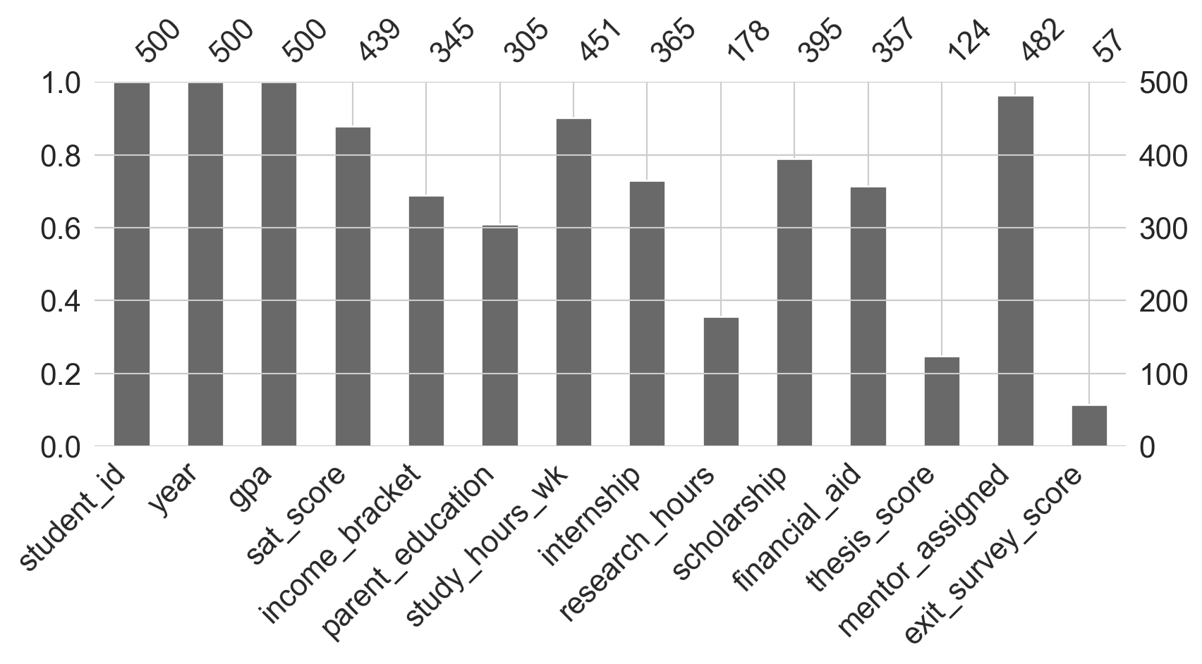

Non-null value counts per column (bar chart).

Matrix — plots a random sample of rows; white streaks mark missing entries. Aligned streaks across columns indicate that variables are missing together.

msno.matrix(students.sample(200, random_state=1), figsize=(11, 4))
plt.show()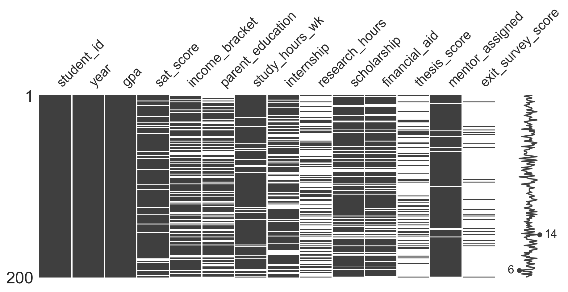

Missing data matrix for 200 randomly sampled rows.

Heatmap — shows the correlation between missingness indicators across pairs of columns. A positive value means the two columns tend to be missing at the same time; a negative value means they are missing at opposite times.

msno.heatmap(students, figsize=(10, 4))
plt.show()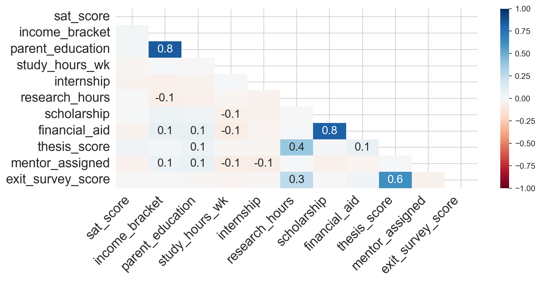

Dendrogram — clusters variables by the similarity of their missingness patterns. Variables linked at distance 0 fully predict one another’s presence.

msno.dendrogram(students, figsize=(10, 4))
plt.tight_layout()
plt.show()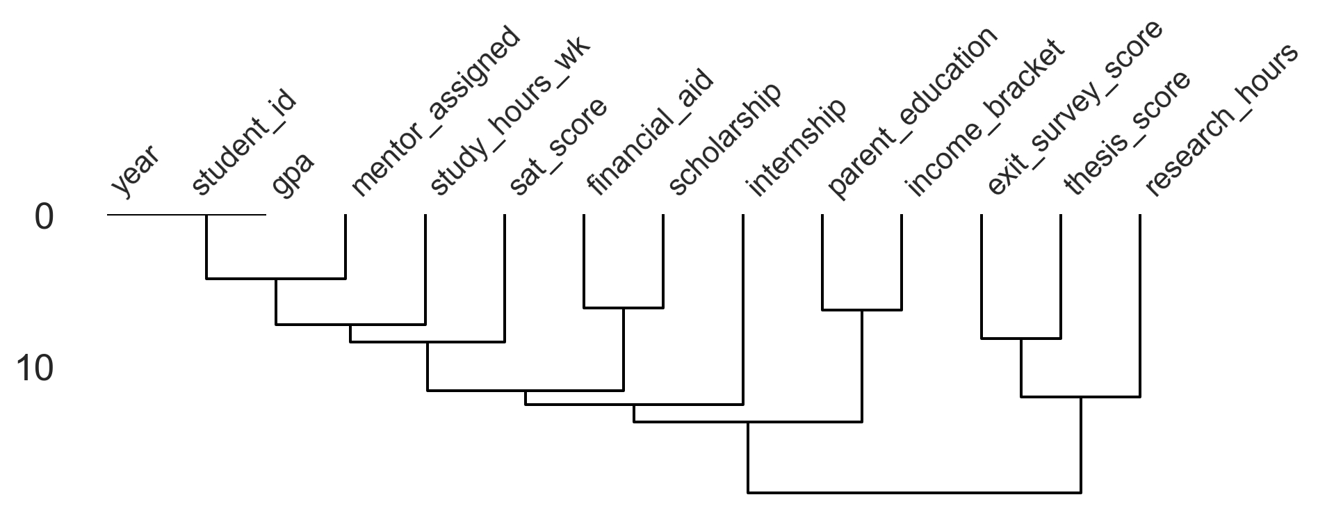

From these plots we can see that scholarship and financial_aid have highly correlated missingness (they were missing together by design), while thesis_score and exit_survey_score are missing as a structural consequence of student year — a clear MNAR pattern.

Handling missing data

Deletion is appropriate when data is MCAR. It is simple but loses information.

# Drop rows with any missing value
students_row_dropped = students.dropna()
print(f"Original rows:       {students.shape[0]}")
print(f"After row deletion:  {students_row_dropped.shape[0]}")

Original rows:       500
After row deletion:  8

# Drop columns with any missing value
students_col_dropped = students.dropna(axis=1)
print(f"Original columns:    {students.shape[1]}")
print(f"After col deletion:  {students_col_dropped.shape[1]}")

Original columns:    14
After col deletion:  3

Row deletion eliminates almost every record here because nearly every row has at least one missing field. Column deletion removes any column with even one null. In practice, targeted deletion — dropping only columns or rows above a missingness threshold — is more useful.

Imputation replaces missing values with plausible substitutes. The fillna method covers the most common strategies:

# Mean imputation for study_hours_wk (MCAR — plausibly random non-response)
students['study_hours_wk'] = students['study_hours_wk'].fillna(
    students['study_hours_wk'].mean()
)

# Forward fill for a time-ordered column (not this dataset, but common in time-series)
# df['col'].ffill()

# Constant fill for remaining numeric columns as a simple baseline
students_imputed = students.bfill(axis=0).fillna(0)
students_imputed.isnull().sum().sum()

Important

Imputation is a deep topic in its own right. The right strategy depends on why data is missing and on the downstream analysis. Always ask: would imputing this value introduce bias?

Duplicate Values

Why duplicates arise

Well-structured data should have a unique identifier for each observation. Duplicates typically arise from data entry errors, merging datasets without deduplication, or system migrations.

We create a small customer dataset that contains both exact duplicates and near-duplicates arising from inconsistent capitalisation.

customers = pd.DataFrame({
    'customer_id': [1001, 1002, 1003, 1004, 1005, 1003, 1006, 1002, 1007, 1004, 1008],
    'name':        ['Alice Johnson', 'bob smith',   'Carol White', 'david lee',
                    'Eve Martinez',  'Carol White', 'Frank Brown', 'Bob Smith',
                    'Grace Kim',     'David Lee',   'Hank Wilson'],
    'email':       ['alice@example.com', 'bob@example.com',   'carol@example.com',
                    'david@example.com', 'eve@example.com',   'carol@example.com',
                    'frank@example.com', 'bob@example.com',   'grace@example.com',
                    'david@example.com', 'hank@example.com'],
    'age':         [28, 34, 45, 29, 52, 45, 38, 34, 41, 29, 55],
    'city':        ['New York', 'los angeles', 'Chicago',     'new york', 'Houston',
                    'Chicago',  'Phoenix',     'Los Angeles', 'Seattle',  'New York', 'Dallas'],
    'spend':       [120.50, 89.99, 245.00, 55.75, 310.20,
                    245.00, 178.40, 89.99,  95.60, 120.00, 430.10],
})
customers

	customer_id	name	email	age	city	spend
0	1001	Alice Johnson	alice@example.com	28	New York	120.50
1	1002	bob smith	bob@example.com	34	los angeles	89.99
2	1003	Carol White	carol@example.com	45	Chicago	245.00
3	1004	david lee	david@example.com	29	new york	55.75
4	1005	Eve Martinez	eve@example.com	52	Houston	310.20
5	1003	Carol White	carol@example.com	45	Chicago	245.00
6	1006	Frank Brown	frank@example.com	38	Phoenix	178.40
7	1002	Bob Smith	bob@example.com	34	Los Angeles	89.99
8	1007	Grace Kim	grace@example.com	41	Seattle	95.60
9	1004	David Lee	david@example.com	29	New York	120.00
10	1008	Hank Wilson	hank@example.com	55	Dallas	430.10

Identifying exact duplicates

dup_count = customers.duplicated().sum()
dup_rows  = customers.loc[customers.duplicated()].index.tolist()
print(f"Exact duplicates: {dup_count}  (rows {dup_rows})")

Exact duplicates: 1  (rows [5])

Near-duplicates from formatting inconsistency

Exact duplicate detection misses rows that differ only in case or whitespace — "bob smith" and "Bob Smith" are the same person. Normalising strings first reveals the full extent of the problem.

customers['name']  = customers['name'].str.strip().str.title()
customers['email'] = customers['email'].str.strip().str.lower()
customers['city']  = customers['city'].str.strip().str.title()

dup_count = customers.duplicated().sum()
dup_rows  = customers.loc[customers.duplicated()].index.tolist()
print(f"Duplicates after normalisation: {dup_count}  (rows {dup_rows})")

Duplicates after normalisation: 2  (rows [5, 7])

Removing duplicates

The simplest resolution is deletion — keep the first occurrence.

customers_clean = customers.drop_duplicates()
print(f"Rows after deduplication: {len(customers_clean)}")

Rows after deduplication: 9

When we want to maximise information, we can aggregate rather than delete. Here we sum spend across duplicate customer IDs and take the first value for all other fields.

customers_agg = (
    customers
    .groupby('customer_id', sort=False)
    .agg({'name': 'first', 'email': 'first', 'age': 'mean', 'city': 'first', 'spend': 'sum'})
    .reset_index()
)
customers_agg

	customer_id	name	email	age	city	spend
0	1001	Alice Johnson	alice@example.com	28.0	New York	120.50
1	1002	Bob Smith	bob@example.com	34.0	Los Angeles	179.98
2	1003	Carol White	carol@example.com	45.0	Chicago	490.00
3	1004	David Lee	david@example.com	29.0	New York	175.75
4	1005	Eve Martinez	eve@example.com	52.0	Houston	310.20
5	1006	Frank Brown	frank@example.com	38.0	Phoenix	178.40
6	1007	Grace Kim	grace@example.com	41.0	Seattle	95.60
7	1008	Hank Wilson	hank@example.com	55.0	Dallas	430.10

Inconsistent Data Types

Pandas infers column types when loading a file, but inference is not always correct. Wrong types break operations silently — averaging a column of numbers stored as strings produces an error, and comparing dates stored as text gives alphabetical rather than chronological ordering. The goal is for every column to have a type that matches its meaning.

Useful inspection tools: dtypes, info(), head(), and unique().

example_df = pd.DataFrame({
    "date":    ["2024-01-01", "2024-01-02", "2024-01-03"],
    "price":   ["1.10", "2.20", "3.30"],
    "in_stock": ["True", "False", "True"],
})
print(example_df.dtypes)

date        object
price       object
in_stock    object
dtype: object

All three columns are read as object (string). Each needs to be coerced to its correct type.

Dates stored as strings

print(f"Before: {example_df['date'].dtype}")
example_df['date'] = pd.to_datetime(example_df['date'])
print(f"After:  {example_df['date'].dtype}")

Before: object
After:  datetime64[ns]

Numbers stored as strings

print(f"Before: {example_df['price'].dtype}")
example_df['price'] = pd.to_numeric(example_df['price'])
print(f"After:  {example_df['price'].dtype}")

Before: object
After:  float64

Booleans stored as strings

print(f"Before: {example_df['in_stock'].dtype}")
example_df['in_stock'] = (
    example_df['in_stock'].str.strip().str.lower()
    .map({"true": True, "false": False})
    .astype("boolean")
)
print(f"After:  {example_df['in_stock'].dtype}")

Before: object
After:  boolean

Mixed date formats

Hand-prepared data often contains dates written in multiple formats within the same column.

mixed_df = pd.DataFrame({
    "date":    ["2024-01-15", "21-12-2001", "December 21, 2001", "01/02/2024", "2018-03-04"],
    "active":  ["True", "false", "true", "no", "yes"],
})

mixed_df['date'] = pd.to_datetime(mixed_df['date'], format="mixed")
mixed_df['active'] = (
    mixed_df['active'].str.strip().str.lower()
    .map({"true": True, "false": False, "yes": True, "no": False})
    .astype("boolean")
)
mixed_df

	date	active
0	2024-01-15	True
1	2001-12-21	False
2	2001-12-21	True
3	2024-01-02	False
4	2018-03-04	True

When loading CSVs you can direct pandas to parse date columns at load time with parse_dates=[...], or specify exact formats via pd.to_datetime(..., format='...'). Use errors='coerce' to turn unparseable entries into NaT rather than raising an exception — this makes it easy to spot remaining problems.

# Day-first strings; invalid entries silently become NaT
pd.to_datetime(
    pd.Series(["15/03/2024", "02/04/2024", "not a date"]),
    dayfirst=True,
    errors="coerce",
)

0   2024-03-15
1   2024-04-02
2          NaT
dtype: datetime64[ns]

Invalid Values

Invalid values are not missing: they appear as real entries but violate domain constraints — an age of 200, a negative count, a temperature of −999 (a common sentinel). They differ from outliers, which may be legitimate extremes. Invalid values are especially dangerous because they do not produce errors; they propagate silently through calculations.

ages = pd.Series([34, 200, 28, -1, 45, 130])
invalid_mask = (ages < 0) | (ages > 120)
print("Invalid entries:\n", ages[invalid_mask])

Invalid entries:
 1    200
3     -1
5    130
dtype: int64

To handle them: define rules from a data dictionary or domain knowledge, flag rows using boolean masks, then drop, replace, or convert to NaN and treat as missing. Document every rule — the why matters as much as the code.

ages_clean = ages.where(~invalid_mask, other=np.nan)
print("After cleaning:\n", ages_clean)

After cleaning:
 0    34.0
1     NaN
2    28.0
3     NaN
4    45.0
5     NaN
dtype: float64

Labelling Issues

The same category can appear under multiple labels: "NYC", "nyc", and "New York" all refer to the same city. Column names can differ across files (customerID vs customer_id), which silently breaks joins and merges.

The fix involves: normalising text with str.strip(), str.lower() / str.title(); building a mapping dictionary from raw labels to canonical ones; and applying it with map() or replace().

city_raw = pd.Series(["  nyc ", "NYC", "New York", "new york", "N.Y.C."])
city_clean = city_raw.str.strip().str.title().replace({"Nyc": "New York", "N.Y.C.": "New York"})
city_clean

0    New York
1    New York
2    New York
3    New York
4    New York
dtype: object

For analysis, maintain a single canonical vocabulary per variable and keep a small “codebook” you can reuse across scripts.