Linear Algebra

An introduction to the key linear algebra definitions and results used in statistics, including vectors, matrices, matrix inverses, projections, and the matrix derivation of the OLS estimator.

ImportantLearning Objectives

• Understand vectors, matrices, and the fundamental operations on them.
• Identify special matrix structures: symmetric, orthogonal, and positive definite.
• Compute and interpret matrix inverses and understand when they exist.
• Define eigenvalues and eigenvectors and understand their role in statistics.
• Set up the linear regression problem in matrix form and derive the OLS estimator.
• Understand the hat matrix and its geometric interpretation.

import numpy as np
import matplotlib.pyplot as plt
import matplotlib.patches as mpatches
import seaborn as sns

sns.set_style('whitegrid')
sns.set_palette('Set2')

Vectors

Definition

A vector is an ordered list of real numbers. A column vector \(\mathbf{v} \in \mathbb{R}^n\) is written:

\[ \mathbf{v} = \begin{pmatrix} v_1 \\ v_2 \\ \vdots \\ v_n \end{pmatrix}. \]

Geometrically, a vector in \(\mathbb{R}^n\) represents a point (or a direction) in \(n\)-dimensional space.

Vector Operations

Addition and scalar multiplication work element-wise:

\[ \mathbf{u} + \mathbf{v} = \begin{pmatrix} u_1 + v_1 \\ \vdots \\ u_n + v_n \end{pmatrix}, \qquad c\,\mathbf{v} = \begin{pmatrix} c v_1 \\ \vdots \\ c v_n \end{pmatrix}. \]

The inner product (dot product) of two vectors \(\mathbf{u}, \mathbf{v} \in \mathbb{R}^n\) is the scalar:

\[ \langle \mathbf{u}, \mathbf{v} \rangle = \mathbf{u}^\top \mathbf{v} = \sum_{i=1}^n u_i v_i. \]

Two vectors are orthogonal if their inner product is zero: \(\mathbf{u}^\top \mathbf{v} = 0\).

The Euclidean norm (length) of a vector is:

\[ \|\mathbf{v}\| = \sqrt{\mathbf{v}^\top \mathbf{v}} = \sqrt{\sum_{i=1}^n v_i^2}. \]

A vector with \(\|\mathbf{v}\| = 1\) is called a unit vector.

u = np.array([1.0, 2.0, 3.0])
v = np.array([4.0, -1.0, 2.0])

print("Inner product:", np.dot(u, v))
print("Norm of u:", np.linalg.norm(u))
print("Orthogonal?", np.isclose(np.dot(u, v), 0))

Inner product: 8.0
Norm of u: 3.7416573867739413
Orthogonal? False

Linear Combinations and Span

A linear combination of vectors \(\mathbf{v}_1, \ldots, \mathbf{v}_k\) is any vector of the form \(c_1 \mathbf{v}_1 + \cdots + c_k \mathbf{v}_k\). The span of a set of vectors is the collection of all their linear combinations.

ImportantLinear Independence

Vectors \(\mathbf{v}_1, \ldots, \mathbf{v}_k\) are linearly independent if the only solution to \[c_1 \mathbf{v}_1 + \cdots + c_k \mathbf{v}_k = \mathbf{0}\] is \(c_1 = \cdots = c_k = 0\). Otherwise they are linearly dependent, meaning at least one vector can be written as a linear combination of the others.

Linear independence is central to regression: if the predictor variables are linearly dependent, the design matrix loses rank and we cannot uniquely estimate coefficients.

Matrices

Definition and Basic Operations

A matrix \(\mathbf{A} \in \mathbb{R}^{m \times n}\) is a rectangular array with \(m\) rows and \(n\) columns:

\[ \mathbf{A} = \begin{pmatrix} a_{11} & a_{12} & \cdots & a_{1n} \\ a_{21} & a_{22} & \cdots & a_{2n} \\ \vdots & & \ddots & \vdots \\ a_{m1} & a_{m2} & \cdots & a_{mn} \end{pmatrix}. \]

Addition and scalar multiplication are element-wise (matrices must have the same shape for addition). Matrix multiplication \(\mathbf{A}\mathbf{B}\) requires the inner dimensions to match: if \(\mathbf{A} \in \mathbb{R}^{m \times k}\) and \(\mathbf{B} \in \mathbb{R}^{k \times n}\) then \(\mathbf{C} = \mathbf{A}\mathbf{B} \in \mathbb{R}^{m \times n}\) with entries:

\[ c_{ij} = \sum_{l=1}^k a_{il}\, b_{lj}. \]

Note that matrix multiplication is not commutative in general: \(\mathbf{A}\mathbf{B} \neq \mathbf{B}\mathbf{A}\).

Transpose

The transpose of \(\mathbf{A} \in \mathbb{R}^{m \times n}\) is \(\mathbf{A}^\top \in \mathbb{R}^{n \times m}\), obtained by swapping rows and columns: \((A^\top)_{ij} = a_{ji}\).

Key properties of the transpose:

\[ (\mathbf{A}^\top)^\top = \mathbf{A}, \qquad (\mathbf{A} + \mathbf{B})^\top = \mathbf{A}^\top + \mathbf{B}^\top, \qquad (\mathbf{A}\mathbf{B})^\top = \mathbf{B}^\top \mathbf{A}^\top. \]

The last identity is the reversal rule for transposes, and appears constantly in regression derivations.

A = np.array([[1, 2, 3],
              [4, 5, 6]])
B = np.array([[7, 8],
              [9, 10],
              [11, 12]])

C = A @ B         # matrix multiplication
print("A @ B:\n", C)
print("(A @ B).T:\n", C.T)
print("B.T @ A.T:\n", B.T @ A.T)   # should match (AB)^T = B^T A^T

A @ B:
 [[ 58  64]
 [139 154]]
(A @ B).T:
 [[ 58 139]
 [ 64 154]]
B.T @ A.T:
 [[ 58 139]
 [ 64 154]]

Special Matrices

Identity Matrix

The identity matrix \(\mathbf{I}_n \in \mathbb{R}^{n \times n}\) has ones on the diagonal and zeros elsewhere. It satisfies \(\mathbf{A}\mathbf{I} = \mathbf{I}\mathbf{A} = \mathbf{A}\) for any compatible matrix \(\mathbf{A}\).

Diagonal Matrix

A diagonal matrix has non-zero entries only on the main diagonal. Diagonal matrices are easy to invert: if \(\mathbf{D} = \mathrm{diag}(d_1, \ldots, d_n)\) with all \(d_i \neq 0\), then \(\mathbf{D}^{-1} = \mathrm{diag}(1/d_1, \ldots, 1/d_n)\).

Symmetric Matrix

A matrix is symmetric if \(\mathbf{A}^\top = \mathbf{A}\), i.e. \(a_{ij} = a_{ji}\) for all \(i, j\). Many important matrices in statistics are symmetric: covariance matrices, Gram matrices \(\mathbf{X}^\top \mathbf{X}\), and the hat matrix \(\mathbf{H}\).

Orthogonal Matrix

A square matrix \(\mathbf{Q}\) is orthogonal if its columns are orthonormal (mutually orthogonal unit vectors), which implies:

\[ \mathbf{Q}^\top \mathbf{Q} = \mathbf{Q}\mathbf{Q}^\top = \mathbf{I}, \quad \text{i.e.} \quad \mathbf{Q}^{-1} = \mathbf{Q}^\top. \]

Orthogonal matrices preserve norms: \(\|\mathbf{Q}\mathbf{v}\| = \|\mathbf{v}\|\). They arise in eigendecompositions and in the geometric interpretation of least squares.

Rank and Invertibility

Rank

The rank of a matrix \(\mathbf{A} \in \mathbb{R}^{m \times n}\) is the maximum number of linearly independent columns (equivalently, rows). We always have \(\mathrm{rank}(\mathbf{A}) \leq \min(m, n)\).

• \(\mathbf{A}\) has full column rank if \(\mathrm{rank}(\mathbf{A}) = n\) (all columns are linearly independent).
• \(\mathbf{A}\) has full row rank if \(\mathrm{rank}(\mathbf{A}) = m\).

X = np.array([[1, 2, 3],
              [4, 5, 6],
              [7, 8, 9]])   # rank-deficient: row 3 = row 1 + row 2 up to constant

print("Rank:", np.linalg.matrix_rank(X))

X_full = np.array([[1, 0, 0],
                   [0, 1, 0],
                   [0, 0, 1]])
print("Rank (identity):", np.linalg.matrix_rank(X_full))

Rank: 2
Rank (identity): 3

Matrix Inverse

For a square matrix \(\mathbf{A} \in \mathbb{R}^{n \times n}\), the inverse \(\mathbf{A}^{-1}\) satisfies:

\[ \mathbf{A}\mathbf{A}^{-1} = \mathbf{A}^{-1}\mathbf{A} = \mathbf{I}_n. \]

ImportantConditions for Invertibility

A square matrix \(\mathbf{A} \in \mathbb{R}^{n \times n}\) is invertible (non-singular) if and only if any of the following equivalent conditions hold:

1. \(\mathrm{rank}(\mathbf{A}) = n\) (full rank).
2. \(\det(\mathbf{A}) \neq 0\).
3. All eigenvalues of \(\mathbf{A}\) are non-zero.
4. The columns of \(\mathbf{A}\) are linearly independent.

Key properties of the inverse:

\[ (\mathbf{A}^{-1})^{-1} = \mathbf{A}, \qquad (\mathbf{A}\mathbf{B})^{-1} = \mathbf{B}^{-1}\mathbf{A}^{-1}, \qquad (\mathbf{A}^\top)^{-1} = (\mathbf{A}^{-1})^\top. \]

The reversal rule \((\mathbf{A}\mathbf{B})^{-1} = \mathbf{B}^{-1}\mathbf{A}^{-1}\) mirrors the reversal rule for transposes.

A = np.array([[2.0, 1.0],
              [5.0, 3.0]])

A_inv = np.linalg.inv(A)
print("A_inv:\n", A_inv)
print("A @ A_inv:\n", np.round(A @ A_inv, 10))  # should be identity

A_inv:
 [[ 3. -1.]
 [-5.  2.]]
A @ A_inv:
 [[ 1.  0.]
 [-0.  1.]]

Quadratic Forms and Positive Definiteness

A quadratic form associated with a symmetric matrix \(\mathbf{A} \in \mathbb{R}^{n \times n}\) is the scalar-valued function:

\[ Q(\mathbf{v}) = \mathbf{v}^\top \mathbf{A} \mathbf{v} = \sum_{i=1}^n \sum_{j=1}^n a_{ij} v_i v_j. \]

Quadratic forms arise throughout statistics — for example, the OLS residual sum of squares is \(\mathrm{RSS} = \mathbf{e}^\top \mathbf{e}\) and the Mahalanobis distance is \((\mathbf{x} - \boldsymbol{\mu})^\top \boldsymbol{\Sigma}^{-1} (\mathbf{x} - \boldsymbol{\mu})\).

ImportantPositive Definiteness

A symmetric matrix \(\mathbf{A}\) is:

• Positive definite (PD) if \(\mathbf{v}^\top \mathbf{A} \mathbf{v} > 0\) for all \(\mathbf{v} \neq \mathbf{0}\).
• Positive semi-definite (PSD) if \(\mathbf{v}^\top \mathbf{A} \mathbf{v} \geq 0\) for all \(\mathbf{v}\).

Equivalently, \(\mathbf{A}\) is PD iff all its eigenvalues are strictly positive, and PSD iff all eigenvalues are non-negative.

The Gram matrix \(\mathbf{X}^\top \mathbf{X}\) is always PSD, and is PD (hence invertible) when \(\mathbf{X}\) has full column rank — a crucial condition for OLS to have a unique solution.

Eigenvalues and Eigenvectors

Definition

For a square matrix \(\mathbf{A} \in \mathbb{R}^{n \times n}\), a non-zero vector \(\mathbf{q}\) and scalar \(\lambda\) satisfying:

\[ \mathbf{A}\mathbf{q} = \lambda \mathbf{q} \]

are called an eigenvector and its associated eigenvalue, respectively. The eigenvalue equation says that \(\mathbf{A}\) stretches (or reflects) \(\mathbf{q}\) by factor \(\lambda\) without changing its direction.

Eigenvalues are found by solving the characteristic equation \(\det(\mathbf{A} - \lambda \mathbf{I}) = 0\).

Eigendecomposition

A symmetric matrix \(\mathbf{A} \in \mathbb{R}^{n \times n}\) always has \(n\) real eigenvalues \(\lambda_1, \ldots, \lambda_n\) and \(n\) orthonormal eigenvectors \(\mathbf{q}_1, \ldots, \mathbf{q}_n\) (by the spectral theorem). We can write:

\[ \mathbf{A} = \mathbf{Q} \boldsymbol{\Lambda} \mathbf{Q}^\top, \]

where \(\mathbf{Q} = [\mathbf{q}_1 \mid \cdots \mid \mathbf{q}_n]\) is orthogonal and \(\boldsymbol{\Lambda} = \mathrm{diag}(\lambda_1, \ldots, \lambda_n)\).

A = np.array([[4.0, 2.0],
              [2.0, 3.0]])

eigenvalues, eigenvectors = np.linalg.eigh(A)   # eigh for symmetric matrices
print("Eigenvalues:", eigenvalues)
print("Eigenvectors (columns):\n", eigenvectors)

# Verify: A q = lambda q for first eigenpair
q1, lam1 = eigenvectors[:, 0], eigenvalues[0]
print("A @ q1:", A @ q1)
print("lam1 * q1:", lam1 * q1)

Eigenvalues: [1.43844719 5.56155281]
Eigenvectors (columns):
 [[ 0.61541221 -0.78820544]
 [-0.78820544 -0.61541221]]
A @ q1: [ 0.88523796 -1.1337919 ]
lam1 * q1: [ 0.88523796 -1.1337919 ]

Trace and Determinant via Eigenvalues

Two convenient identities link eigenvalues to matrix invariants:

\[ \mathrm{tr}(\mathbf{A}) = \sum_{i=1}^n \lambda_i, \qquad \det(\mathbf{A}) = \prod_{i=1}^n \lambda_i. \]

These are useful for understanding properties of the hat matrix later.

Projections

Orthogonal Projection

Given a subspace \(\mathcal{V} \subseteq \mathbb{R}^n\), the orthogonal projection of a vector \(\mathbf{y}\) onto \(\mathcal{V}\) is the unique vector \(\hat{\mathbf{y}} \in \mathcal{V}\) closest to \(\mathbf{y}\) in Euclidean distance:

\[ \hat{\mathbf{y}} = \underset{\mathbf{v} \in \mathcal{V}}{\arg\min}\, \|\mathbf{y} - \mathbf{v}\|^2. \]

The residual \(\mathbf{e} = \mathbf{y} - \hat{\mathbf{y}}\) is orthogonal to every vector in \(\mathcal{V}\).

ImportantProjection Matrix

If \(\mathcal{V} = \mathrm{col}(\mathbf{X})\) (the column space of \(\mathbf{X}\)) and \(\mathbf{X}\) has full column rank, the orthogonal projection onto \(\mathcal{V}\) is the linear map: \[ \hat{\mathbf{y}} = \mathbf{H}\mathbf{y}, \qquad \mathbf{H} = \mathbf{X}(\mathbf{X}^\top \mathbf{X})^{-1}\mathbf{X}^\top. \] \(\mathbf{H}\) is called the hat matrix (or projection matrix).

Properties of Projection Matrices

Any orthogonal projection matrix \(\mathbf{H}\) satisfies two key properties:

1. Symmetric: \(\mathbf{H}^\top = \mathbf{H}\).
2. Idempotent: \(\mathbf{H}^2 = \mathbf{H}\) (projecting twice gives the same result as projecting once).

# Simple 2D projection example
X = np.array([[1.0], [2.0], [3.0]])   # n=3, p=1 (no intercept, for illustration)
H = X @ np.linalg.inv(X.T @ X) @ X.T

print("Symmetric?", np.allclose(H, H.T))
print("Idempotent?", np.allclose(H @ H, H))
print("Trace of H:", np.trace(H))     # = number of columns in X

Symmetric? True
Idempotent? True
Trace of H: 0.9999999999999999

The trace of the hat matrix equals the number of columns in \(\mathbf{X}\) (i.e. \(p + 1\) for a model with an intercept and \(p\) predictors), which counts the “degrees of freedom” used by the model.

The complementary matrix \(\mathbf{M} = \mathbf{I} - \mathbf{H}\) projects onto the orthogonal complement of \(\mathrm{col}(\mathbf{X})\) and is also symmetric and idempotent. The residual vector in OLS is \(\mathbf{e} = \mathbf{M}\mathbf{y}\).

Linear Regression in Matrix Form

The Design Matrix

Suppose we have \(n\) observations \((y_i, x_{i1}, \ldots, x_{ip})\) for \(i = 1, \ldots, n\). The multiple linear regression model is:

\[ y_i = \beta_0 + \beta_1 x_{i1} + \cdots + \beta_p x_{ip} + \varepsilon_i. \]

Stacking all \(n\) equations, we can write this compactly as:

\[ \mathbf{y} = \mathbf{X}\boldsymbol{\beta} + \boldsymbol{\varepsilon}, \]

where:

\[ \mathbf{y} = \begin{pmatrix} y_1 \\ \vdots \\ y_n \end{pmatrix} \in \mathbb{R}^n, \quad \mathbf{X} = \begin{pmatrix} 1 & x_{11} & \cdots & x_{1p} \\ \vdots & \vdots & & \vdots \\ 1 & x_{n1} & \cdots & x_{np} \end{pmatrix} \in \mathbb{R}^{n \times (p+1)}, \quad \boldsymbol{\beta} = \begin{pmatrix} \beta_0 \\ \beta_1 \\ \vdots \\ \beta_p \end{pmatrix} \in \mathbb{R}^{p+1}. \]

\(\mathbf{X}\) is called the design matrix. The leading column of ones encodes the intercept term.

Deriving the OLS Estimator

Ordinary least squares (OLS) minimises the residual sum of squares:

\[ \mathrm{RSS}(\boldsymbol{\beta}) = \|\mathbf{y} - \mathbf{X}\boldsymbol{\beta}\|^2 = (\mathbf{y} - \mathbf{X}\boldsymbol{\beta})^\top(\mathbf{y} - \mathbf{X}\boldsymbol{\beta}). \]

Expanding the quadratic form:

\[ \mathrm{RSS}(\boldsymbol{\beta}) = \mathbf{y}^\top\mathbf{y} - 2\boldsymbol{\beta}^\top\mathbf{X}^\top\mathbf{y} + \boldsymbol{\beta}^\top\mathbf{X}^\top\mathbf{X}\boldsymbol{\beta}. \]

Taking the gradient with respect to \(\boldsymbol{\beta}\) and setting it to zero:

\[ \frac{\partial\, \mathrm{RSS}}{\partial \boldsymbol{\beta}} = -2\mathbf{X}^\top\mathbf{y} + 2\mathbf{X}^\top\mathbf{X}\boldsymbol{\beta} = \mathbf{0}. \]

This gives the normal equations:

\[ \mathbf{X}^\top \mathbf{X}\,\hat{\boldsymbol{\beta}} = \mathbf{X}^\top \mathbf{y}. \]

When \(\mathbf{X}\) has full column rank, \(\mathbf{X}^\top\mathbf{X}\) is invertible and the unique solution is:

ImportantOLS Estimator

\[ \hat{\boldsymbol{\beta}} = (\mathbf{X}^\top \mathbf{X})^{-1}\mathbf{X}^\top \mathbf{y}. \]

The fitted values are then:

\[ \hat{\mathbf{y}} = \mathbf{X}\hat{\boldsymbol{\beta}} = \mathbf{X}(\mathbf{X}^\top\mathbf{X})^{-1}\mathbf{X}^\top\mathbf{y} = \mathbf{H}\mathbf{y}, \]

confirming that \(\mathbf{H}\) projects \(\mathbf{y}\) onto the column space of \(\mathbf{X}\).

np.random.seed(42)
n = 50

# True model: y = 1 + 2*x + noise
x = np.linspace(0, 5, n)
y = 1 + 2 * x + np.random.normal(0, 1, n)

# Design matrix (intercept + one predictor)
X = np.column_stack([np.ones(n), x])

# OLS via normal equations
XtX = X.T @ X
Xty = X.T @ y
beta_hat = np.linalg.solve(XtX, Xty)   # solve is numerically preferred to inv()
print("beta_hat:", beta_hat)            # should be close to [1, 2]

y_hat = X @ beta_hat
residuals = y - y_hat
print("RSS:", residuals @ residuals)

beta_hat: [1.06444309 1.8840332 ]
RSS: 41.257089755557885

Note that we use np.linalg.solve rather than explicitly computing np.linalg.inv(XtX). Solving the linear system directly is numerically more stable and avoids forming the inverse unnecessarily.

The Hat Matrix and Its Properties

The hat matrix \(\mathbf{H} = \mathbf{X}(\mathbf{X}^\top\mathbf{X})^{-1}\mathbf{X}^\top\) has several properties that matter for regression diagnostics:

Property	Formula	Interpretation
Symmetric	\(\mathbf{H}^\top = \mathbf{H}\)	Projection matrices are self-adjoint
Idempotent	\(\mathbf{H}^2 = \mathbf{H}\)	Projecting twice = projecting once
Trace	\(\mathrm{tr}(\mathbf{H}) = p + 1\)	Degrees of freedom used by the model
Eigenvalues	\(\lambda_i \in \{0, 1\}\)	Consequence of idempotency
Residuals	\(\mathbf{e} = (\mathbf{I} - \mathbf{H})\mathbf{y}\)	Residuals live in the null space of \(\mathbf{X}\)

The diagonal entries \(h_{ii} = [\mathbf{H}]_{ii}\) are called leverage values. They measure how far observation \(i\) is from the centre of the predictor space; high-leverage points have a disproportionate influence on the fitted values.

H = X @ np.linalg.inv(X.T @ X) @ X.T

print("Symmetric?", np.allclose(H, H.T))
print("Idempotent?", np.allclose(H @ H, H))
print("Trace:", np.round(np.trace(H)))    # = p + 1 = 2

leverages = np.diag(H)
fig, ax = plt.subplots(figsize=(8, 3))
ax.stem(x, leverages, markerfmt='C0o', linefmt='C0-', basefmt='k-')
ax.axhline(2 * (2) / n, color='C1', linestyle='--', label=f'2(p+1)/n threshold')
ax.set_xlabel('x')
ax.set_ylabel('Leverage $h_{ii}$')
ax.set_title('Hat Matrix Diagonal (Leverage Values)')
ax.legend()
plt.tight_layout()
plt.show()

Symmetric? True
Idempotent? True
Trace: 2.0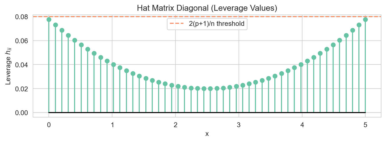

Points at the extremes of the predictor range have the highest leverage — they exert the most pull on the estimated regression line. The conventional threshold for flagging high leverage is \(h_{ii} > 2(p+1)/n\).

Variance of the OLS Estimator

Under the classical OLS assumptions (\(\mathbb{E}[\boldsymbol{\varepsilon}] = \mathbf{0}\), \(\mathrm{Var}(\boldsymbol{\varepsilon}) = \sigma^2 \mathbf{I}\)), the covariance matrix of \(\hat{\boldsymbol{\beta}}\) is:

\[ \mathrm{Var}(\hat{\boldsymbol{\beta}}) = \sigma^2 (\mathbf{X}^\top \mathbf{X})^{-1}. \]

This follows from the general formula \(\mathrm{Var}(\mathbf{A}\mathbf{y}) = \mathbf{A}\,\mathrm{Var}(\mathbf{y})\,\mathbf{A}^\top\) applied with \(\mathbf{A} = (\mathbf{X}^\top\mathbf{X})^{-1}\mathbf{X}^\top\):

\[ \mathrm{Var}(\hat{\boldsymbol{\beta}}) = (\mathbf{X}^\top\mathbf{X})^{-1}\mathbf{X}^\top \cdot \sigma^2\mathbf{I} \cdot \mathbf{X}(\mathbf{X}^\top\mathbf{X})^{-1} = \sigma^2(\mathbf{X}^\top\mathbf{X})^{-1}. \]

The diagonal entries of \((\mathbf{X}^\top\mathbf{X})^{-1}\) (scaled by \(\hat{\sigma}^2\)) give the estimated variances of \(\hat{\beta}_0, \hat{\beta}_1, \ldots, \hat{\beta}_p\), used to construct standard errors and \(t\)-statistics.

sigma2_hat = (residuals @ residuals) / (n - 2)   # unbiased estimate: n - (p+1)
cov_beta = sigma2_hat * np.linalg.inv(X.T @ X)
se_beta = np.sqrt(np.diag(cov_beta))

print("Estimated coefficients:", np.round(beta_hat, 4))
print("Standard errors:", np.round(se_beta, 4))
print("t-statistics:", np.round(beta_hat / se_beta, 4))

Estimated coefficients: [1.0644 1.884 ]
Standard errors: [0.2583 0.089 ]
t-statistics: [ 4.1203 21.1598]

Summary

This chapter developed the matrix language used throughout the regression chapters. The key results are:

• The OLS estimator \(\hat{\boldsymbol{\beta}} = (\mathbf{X}^\top\mathbf{X})^{-1}\mathbf{X}^\top\mathbf{y}\) is derived by minimising RSS, and exists uniquely when \(\mathbf{X}\) has full column rank.
• The fitted values \(\hat{\mathbf{y}} = \mathbf{H}\mathbf{y}\) are the orthogonal projection of \(\mathbf{y}\) onto the column space of \(\mathbf{X}\).
• The hat matrix \(\mathbf{H}\) is symmetric and idempotent with trace \(p+1\); its diagonal entries are leverage values.
• The covariance matrix \(\sigma^2(\mathbf{X}^\top\mathbf{X})^{-1}\) underlies all standard errors and inference procedures in linear regression.