Logistic Regression

Logistic regression in python using the famous Titanic data set.

ImportantLearning Objectives

• Define the logistic regression model.
• Implement logistic regression in python using the famous Titanic classification data set.

# Libraries
import numpy as np
import pandas as pd
import matplotlib.pyplot as plt
import seaborn as sns
from scipy.stats import norm, binom
from scipy.special import expit          # the logistic (sigmoid) function
import statsmodels.formula.api as smf
import statsmodels.api as sm
from statsmodels.stats.anova import anova_lm
from sklearn.metrics import (
    confusion_matrix, ConfusionMatrixDisplay,
    roc_curve, roc_auc_score
)

# Figure styling
sns.set_style('whitegrid')
sns.set_palette('Set2')

Logistic Regression

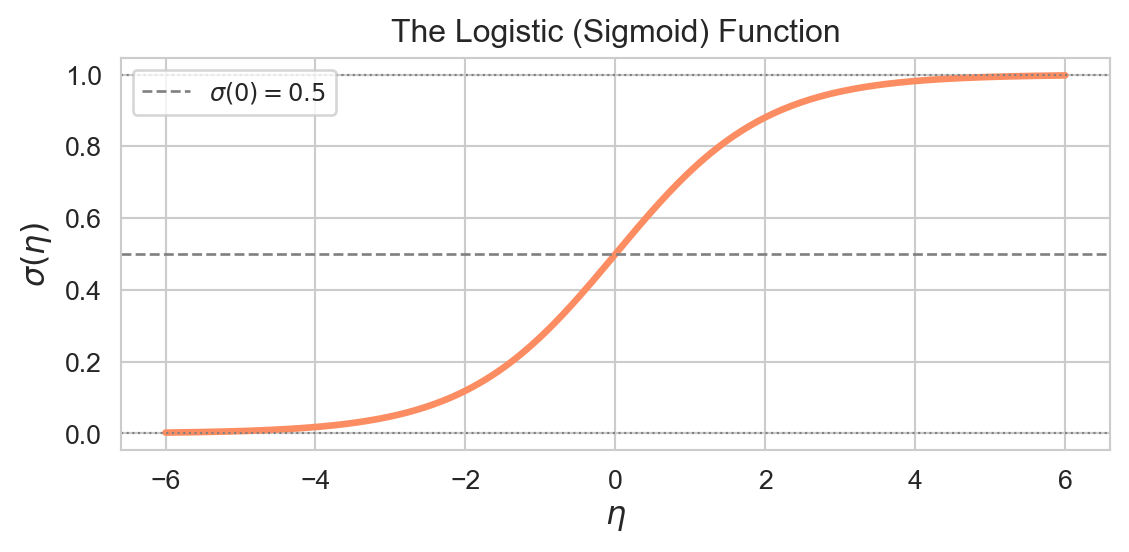
Logistic regression is the GLM for a binary response \(Y_i \in \{0,1\}\). It arises naturally in settings like: did a patient recover? did a loan default? is a species present at a site?

We assume \(Y_i \mid \mathbf{x}_i \sim \text{Bernoulli}(\pi_i)\) and model the log-odds (logit) of \(\pi_i\) as a linear function of the predictors:

\[\log\frac{\pi_i}{1 - \pi_i} = \mathbf{x}_i^\top\boldsymbol{\beta} = \beta_0 + \beta_1 x_{i1} + \cdots + \beta_p x_{ip}.\]

Inverting the logit link gives the logistic (sigmoid) function, which maps any real number to \((0,1)\) and ensures probabilities are always valid:

\[\pi_i = \sigma(\eta_i) = \frac{1}{1 + e^{-\eta_i}}, \quad \eta_i = \mathbf{x}_i^\top\boldsymbol{\beta}.\]

The logistic function maps any real number to the interval (0, 1).

Interpreting Coefficients

Coefficients can be read on three equivalent scales:

Scale	Formula	Interpretation
Log-odds	\(\log\frac{\pi}{1-\pi} = \boldsymbol{x}^\top\boldsymbol{\beta}\)	Linear, unbounded — the model lives here
Odds	\(\frac{\pi}{1-\pi} = e^{\boldsymbol{x}^\top\boldsymbol{\beta}}\)	\(e^{\beta_j}\) is the odds ratio per unit increase in \(x_j\)
Probability	\(\pi = \sigma(\boldsymbol{x}^\top\boldsymbol{\beta})\)	Non-linear; depends on the values of all predictors

If \(\beta_j = 0.5\), then \(e^{0.5} \approx 1.65\): a one-unit increase in \(X_j\) multiplies the odds by \(1.65\). Odds ratios are multiplicative, not additive. If \(\beta_j < 0\), the odds decrease with \(X_j\).

The log-likelihood (also called binary cross-entropy) is:

\[ \ell(\boldsymbol{\beta}) = \sum_{i=1}^n \left[y_i \log \pi_i + (1 - y_i)\log(1 - \pi_i)\right]. \]

A pseudo-\(R^2\) is often computed as McFadden’s \(R^2 = 1 - D/D_0\).

Application: Titanic Survival

We illustrate logistic regression on Titanic passenger data — a classic binary classification problem where \(Y = 1\) indicates survival, with predictors including class, sex, age, and fare.

titanic = (
    sns.load_dataset('titanic')
    [['survived', 'pclass', 'sex', 'age', 'fare', 'embark_town']]
    .dropna()
    .reset_index(drop=True)
)
titanic.head()

	survived	pclass	sex	age	fare	embark_town
0	0	3	male	22.0	7.2500	Southampton
1	1	1	female	38.0	71.2833	Cherbourg
2	1	3	female	26.0	7.9250	Southampton
3	1	1	female	35.0	53.1000	Southampton
4	0	3	male	35.0	8.0500	Southampton

fig, axes = plt.subplots(1, 2, figsize=(9.5, 4))

sex_surv = titanic.groupby('sex')['survived'].mean().reset_index()
sns.barplot(data=sex_surv, x='sex', y='survived', hue='sex', legend=False, ax=axes[0], palette='Set2')
axes[0].set_ylabel('Survival rate')
axes[0].set_title('Survival Rate by Sex')
axes[0].set_ylim(0, 1)

cls_surv = titanic.groupby('pclass', observed=True)['survived'].mean().reset_index()
sns.barplot(data=cls_surv, x='pclass', y='survived', hue='pclass', legend=False, ax=axes[1], palette='Set2')
axes[1].set_ylabel('Survival rate')
axes[1].set_xlabel('Passenger class')
axes[1].set_title('Survival Rate by Passenger Class')
axes[1].set_ylim(0, 1)

plt.suptitle('Titanic: Survival Rates by Demographic', fontsize=13, y=1.02)
plt.tight_layout(); plt.show()

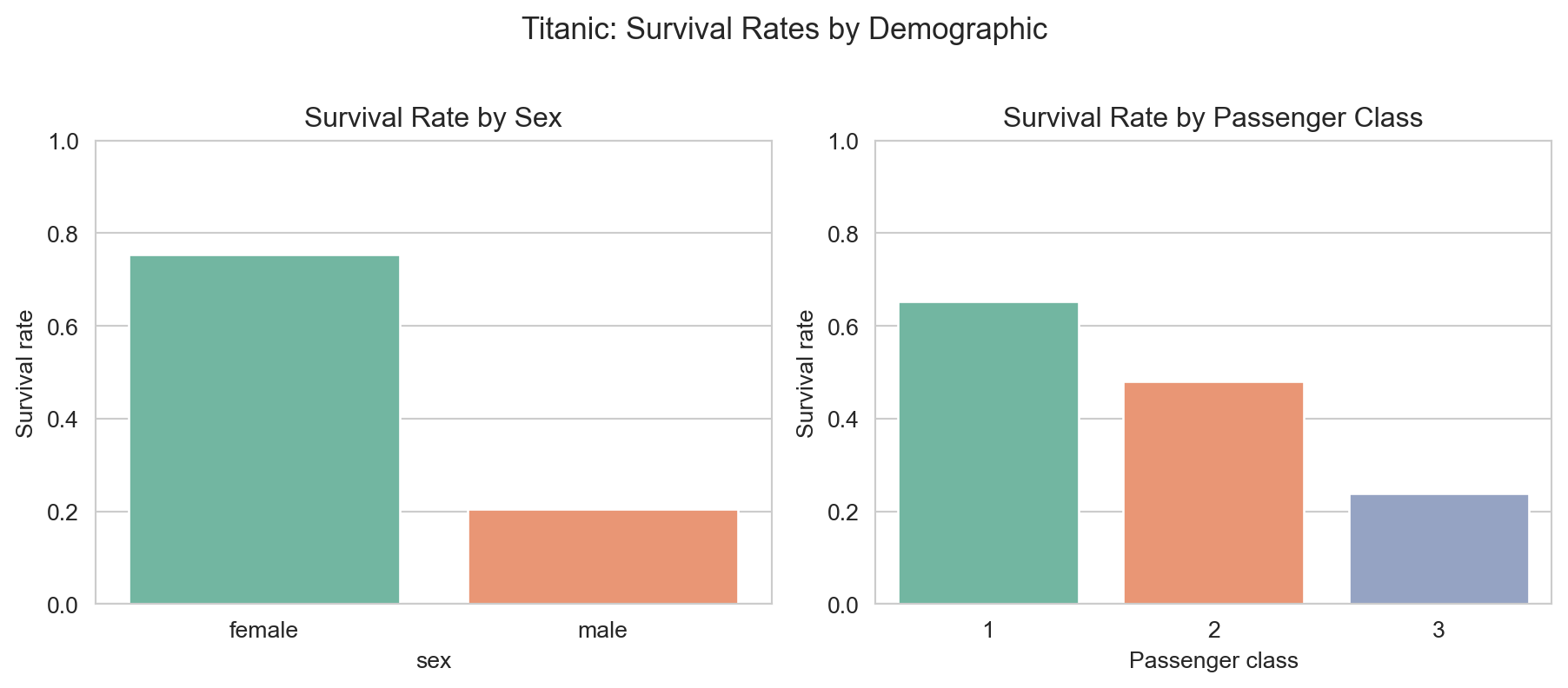
Survival rates by sex and passenger class. Women and first-class passengers had substantially higher survival rates.

fig, ax = plt.subplots(figsize=(9, 4))
for label, grp in titanic.groupby('survived'):
    sns.kdeplot(grp['age'], ax=ax, fill=True, alpha=0.4,
                label='Survived' if label == 1 else 'Did not survive')
ax.set_xlabel('Age (years)')
ax.set_ylabel('Density')
ax.set_title('Age Distribution by Survival Outcome')
ax.legend()
plt.tight_layout(); plt.show()

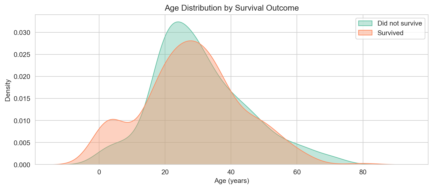
Age distributions for survivors and non-survivors. Children show a somewhat higher survival rate, consistent with the ‘women and children first’ policy.

We fit the model using smf.logit(), which uses the same formula syntax as smf.ols(). Categorical variables are automatically dummy-coded with C(...).

logit1 = smf.logit(
    'survived ~ C(sex) + age + C(pclass) + fare',
    data=titanic
).fit()
print(logit1.summary())

Optimization terminated successfully.
         Current function value: 0.454099
         Iterations 6
                           Logit Regression Results                           
==============================================================================
Dep. Variable:               survived   No. Observations:                  712
Model:                          Logit   Df Residuals:                      706
Method:                           MLE   Df Model:                            5
Date:                Sat, 23 May 2026   Pseudo R-squ.:                  0.3271
Time:                        13:13:39   Log-Likelihood:                -323.32
converged:                       True   LL-Null:                       -480.45
Covariance Type:            nonrobust   LLR p-value:                 8.567e-66
==================================================================================
                     coef    std err          z      P>|z|      [0.025      0.975]
----------------------------------------------------------------------------------
Intercept          3.7150      0.464      7.998      0.000       2.805       4.625
C(sex)[T.male]    -2.5096      0.208    -12.041      0.000      -2.918      -2.101
C(pclass)[T.2]    -1.2682      0.313     -4.055      0.000      -1.881      -0.655
C(pclass)[T.3]    -2.5336      0.328     -7.728      0.000      -3.176      -1.891
age               -0.0369      0.008     -4.769      0.000      -0.052      -0.022
fare               0.0005      0.002      0.230      0.818      -0.004       0.005
==================================================================================

Key fields in the output:

Output	Meaning
Log-Likelihood	Value of \(\ell(\hat{\boldsymbol{\beta}})\) at convergence — higher is better
LL-Null	Log-likelihood of intercept-only model
Pseudo \(R^2\)	McFadden’s: \(1 - \ell(\hat{\boldsymbol{\beta}})/\ell_0\)
Coef	Log-odds coefficients \(\hat{\beta}_j\)
\(P > |z|\)	Wald test \(p\)-value for \(H_0: \beta_j = 0\)
\([0.025,\, 0.975]\)	95% confidence interval on the log-odds scale

Standard errors and tests are based on the Wald statistic \(z = \hat{\beta}_j / \widehat{\text{SE}}(\hat{\beta}_j) \approx \mathcal{N}(0,1)\), a large-sample result from maximum likelihood theory.

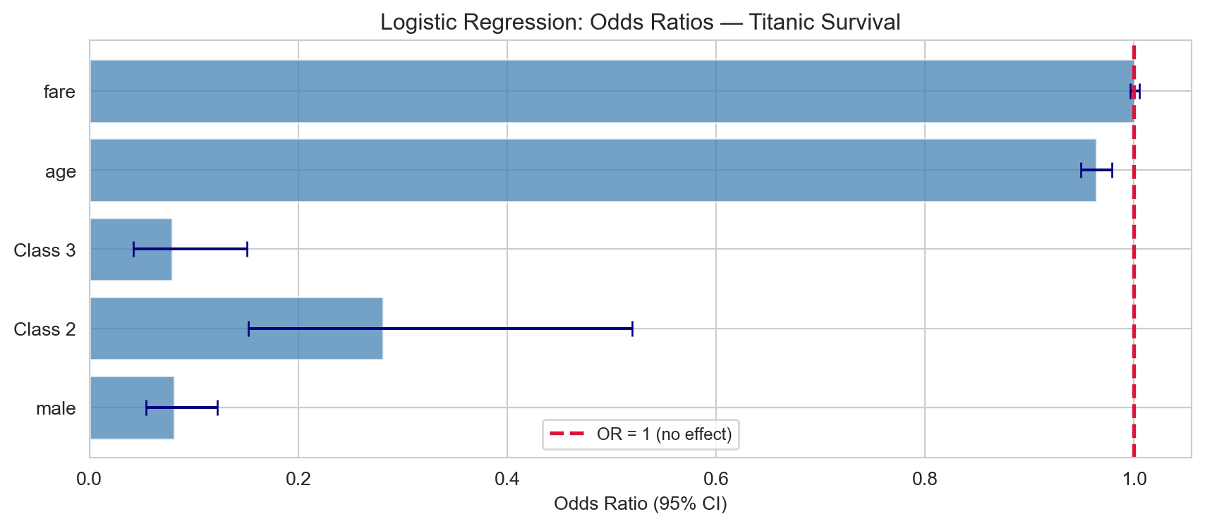
Odds ratios with 95% confidence intervals for the Titanic logistic regression. An odds ratio > 1 means increased odds of survival; < 1 means decreased odds.

We can predict probabilities for individual passengers using logit1.predict(). The coefficient table lives on the log-odds scale, but for communication we usually want probabilities:

newdata = pd.DataFrame({
    'sex':    ['female', 'male'],
    'age':    [30, 30],
    'pclass': [1, 3],
    'fare':   [50, 10]
})
probs = logit1.predict(newdata)
for i, row in newdata.iterrows():
    print(f"  {row['sex']:6s}, age {row['age']}, class {row['pclass']}, "
          f"fare {row['fare']:.0f}: P(survive) = {probs[i]:.3f}")

  female, age 30, class 1, fare 50: P(survive) = 0.933
  male  , age 30, class 3, fare 10: P(survive) = 0.081

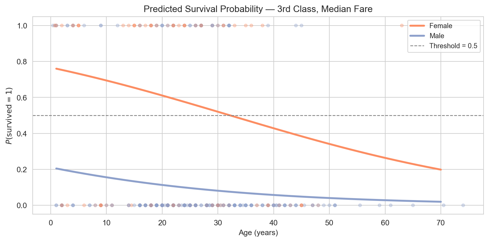
A 30-year-old female in first class has a high predicted survival probability; a 30-year-old male in third class has a much lower one — consistent with the historical record.

Predicted survival probability as a function of age, stratified by sex, for a third-class passenger with median fare. The logistic curve is clearly visible.

Classification Performance

ImportantIn-sample evaluation

The classification metrics below are computed on the same data used to fit the model, giving an optimistic picture of predictive performance. In a prediction-focused workflow you would split data into training and test sets before reporting these metrics. Here our primary goal is inference — understanding which predictors are associated with survival — and the classification metrics illustrate how a fitted logistic regression translates into a classifier.

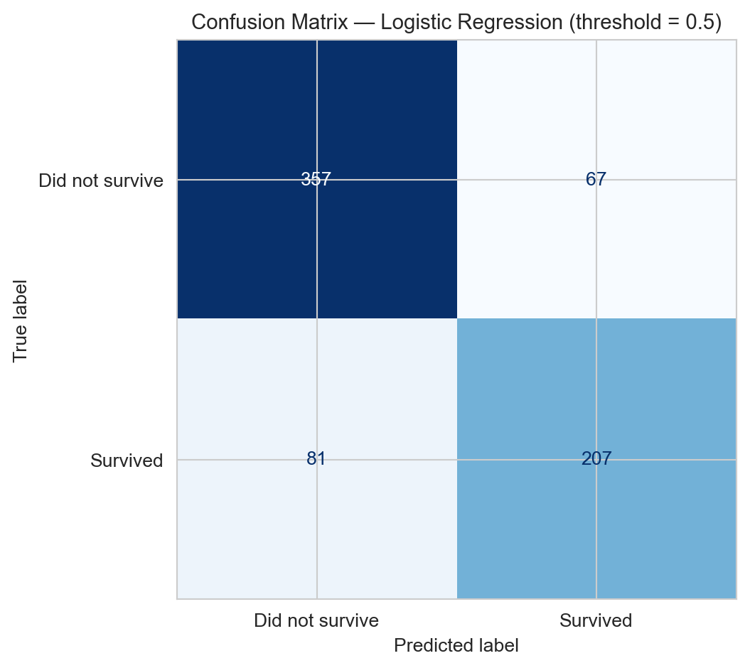
We classify \(\hat{Y}_i = 1\) if \(\hat{\pi}_i > 0.5\) and summarise performance with the confusion matrix and ROC curve.

pi_hat = logit1.predict()
y_pred = (pi_hat >= 0.5).astype(int)
y_true = titanic['survived'].values
acc = (y_pred == y_true).mean()
print(f"Accuracy: {acc:.3f}")

Accuracy: 0.792

Confusion matrix for the logistic regression model at threshold 0.5 (in-sample).

The ROC curve plots the true positive rate (sensitivity) against the false positive rate (1 - specificity) as the threshold varies from 1 to 0. The AUC (area under the ROC curve) measures overall discriminative ability: AUC = 1 is perfect; AUC = 0.5 is a random classifier.

ROC curve for the logistic regression model (in-sample). AUC substantially above 0.5 indicates good discriminative power.

We can test whether adding embark_town improves the model using the LRT:

logit2 = smf.logit(
    'survived ~ C(sex) + age + C(pclass) + fare + C(embark_town)',
    data=titanic
).fit(disp=False)

G2 = 2 * (logit2.llf - logit1.llf)
dof = logit2.df_model - logit1.df_model
from scipy.stats import chi2
p_lrt = chi2.sf(G2, df=dof)
print(f"LRT G² = {G2:.3f},  df = {int(dof)},  p-value = {p_lrt:.4f}")

LRT G² = 3.964,  df = 2,  p-value = 0.1378

print(f"{'Model':<30} {'AIC':>8} {'BIC':>8} {'Pseudo R²':>10}")
print("-" * 58)
for name, m in [('Without embark_town', logit1), ('With embark_town', logit2)]:
    pr2 = 1 - m.llf / m.llnull
    print(f"{name:<30} {m.aic:>8.2f} {m.bic:>8.2f} {pr2:>10.4f}")

Model                               AIC      BIC  Pseudo R²
----------------------------------------------------------
Without embark_town              658.64   686.05     0.3271
With embark_town                 658.67   695.22     0.3312

References