Generalized Linear Models

In this note we define the Generalized Linear Models, link functions and several specific implementations including logistic regression and Poisson regression.

ImportantLearning Objectives

• Understand the limitations of linear regression when the response is not continuous.
• Introduce the Generalized Linear Model (GLM) framework: exponential family, link functions, and maximum likelihood estimation.

# Libraries
import numpy as np
import pandas as pd
import matplotlib.pyplot as plt
import seaborn as sns
from scipy.stats import norm, binom
from scipy.special import expit          # the logistic (sigmoid) function
import statsmodels.formula.api as smf
import statsmodels.api as sm
from statsmodels.stats.anova import anova_lm
from sklearn.metrics import (
    confusion_matrix, ConfusionMatrixDisplay,
    roc_curve, roc_auc_score
)

# Figure styling
sns.set_style('whitegrid')
sns.set_palette('Set2')

The Limits of Linear Regression

The MLR model assumes \(Y_i \sim \mathcal{N}(\mu_i, \sigma^2)\) with \(\mu_i = \mathbf{x}_i^\top \boldsymbol{\beta}\), so the mean is modelled as an unrestricted linear combination of predictors. This breaks down for many common response types:

Common response types incompatable with MLR.

Response type	Example	Problem with linear regression
Binary	Patient survived / died	Predictions outside \([0, 1]\); errors not normal
Count	Number of insurance claims	Must be non-negative; variance grows with mean
Proportion	Percentage of votes won	Bounded in \([0, 1]\); heteroscedastic
Positive continuous	Hospital length of stay	Right-skewed; errors non-normal

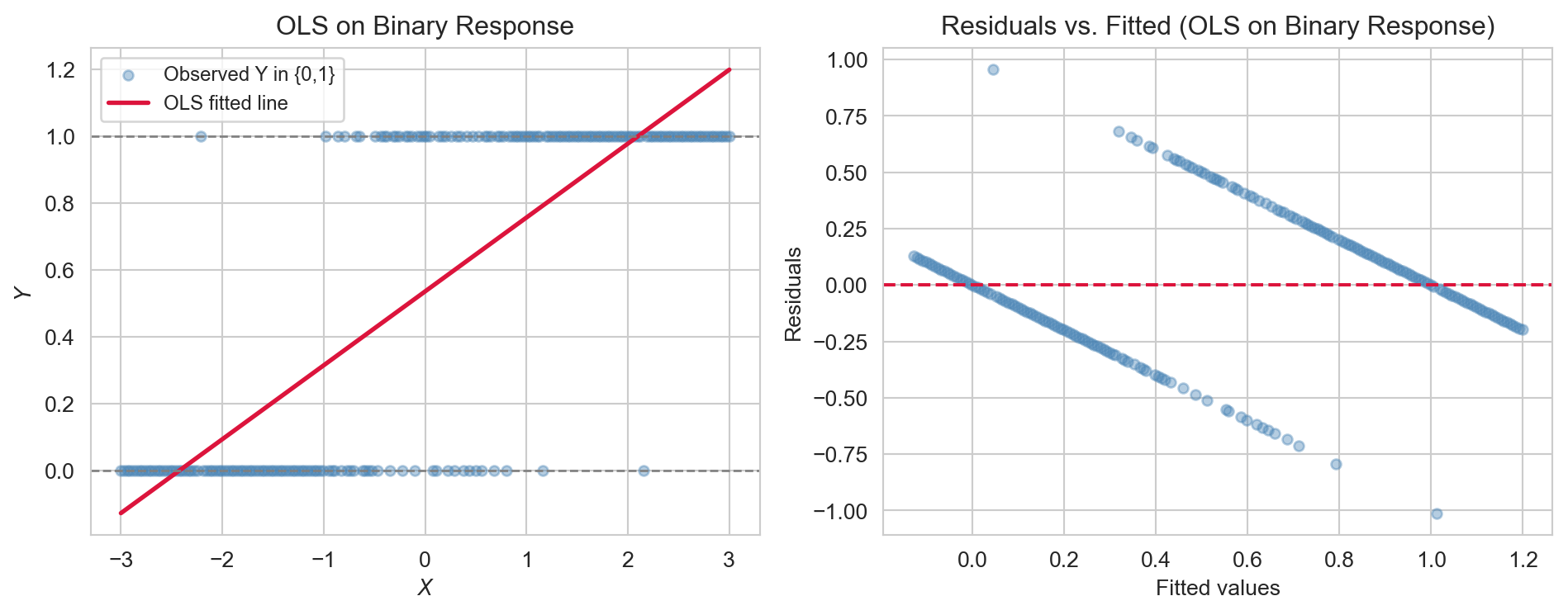
As a concrete example, suppose we want to predict whether a Titanic passenger survived (\(Y_i \in \{0,1\}\)) from their characteristics. We want to model \(P(Y_i = 1 \mid \mathbf{x}_i)\), but fitting OLS directly produces predictions outside \([0,1]\) and clearly non-normal residuals.

OLS fitted to a binary outcome: predicted values fall outside [0, 1] for extreme predictor values, and the residuals are clearly non-normal.

The Generalized Linear Model

ImportantGeneralized Linear Model (GLM)

A GLM extends linear regression by relaxing the normality assumption. It has three components:

1. Random component: the response \(Y_i\) follows a distribution from the exponential family with mean \(\mu_i = \mathbb{E}[Y_i]\).
2. Systematic component: a linear predictor \(\eta_i = \mathbf{x}_i^\top \boldsymbol{\beta}\).
3. Link function \(g\): connects the mean to the linear predictor, \(g(\mu_i) = \eta_i\).

The key idea is that we no longer model \(\mu_i\) directly as a linear combination. Instead we model a transformation of \(\mu_i\) linearly: \(g(\mu_i) = \eta_i = \mathbf{x}_i^\top \boldsymbol{\beta}\). The link function ensures that \(\mu_i\) stays in the valid range for the chosen distribution.

The Exponential Family

A distribution belongs to the exponential family if its probability density/mass function can be written as

\[ f(y \mid \theta, \phi) = \exp\!\left\{\frac{y\theta - b(\theta)}{a(\phi)} + c(y, \phi)\right\}, \]

where \(\theta\) is the canonical parameter, \(\phi\) is the dispersion parameter, and \(b(\cdot)\), \(a(\cdot)\), \(c(\cdot)\) are known functions. Two important properties follow: \(\mu = \mathbb{E}[Y] = b'(\theta)\) and \(\text{Var}(Y) = b''(\theta)\,a(\phi)\) — variance is a function of the mean.

Distribution	Response type	Canonical link \(g(\mu)\)
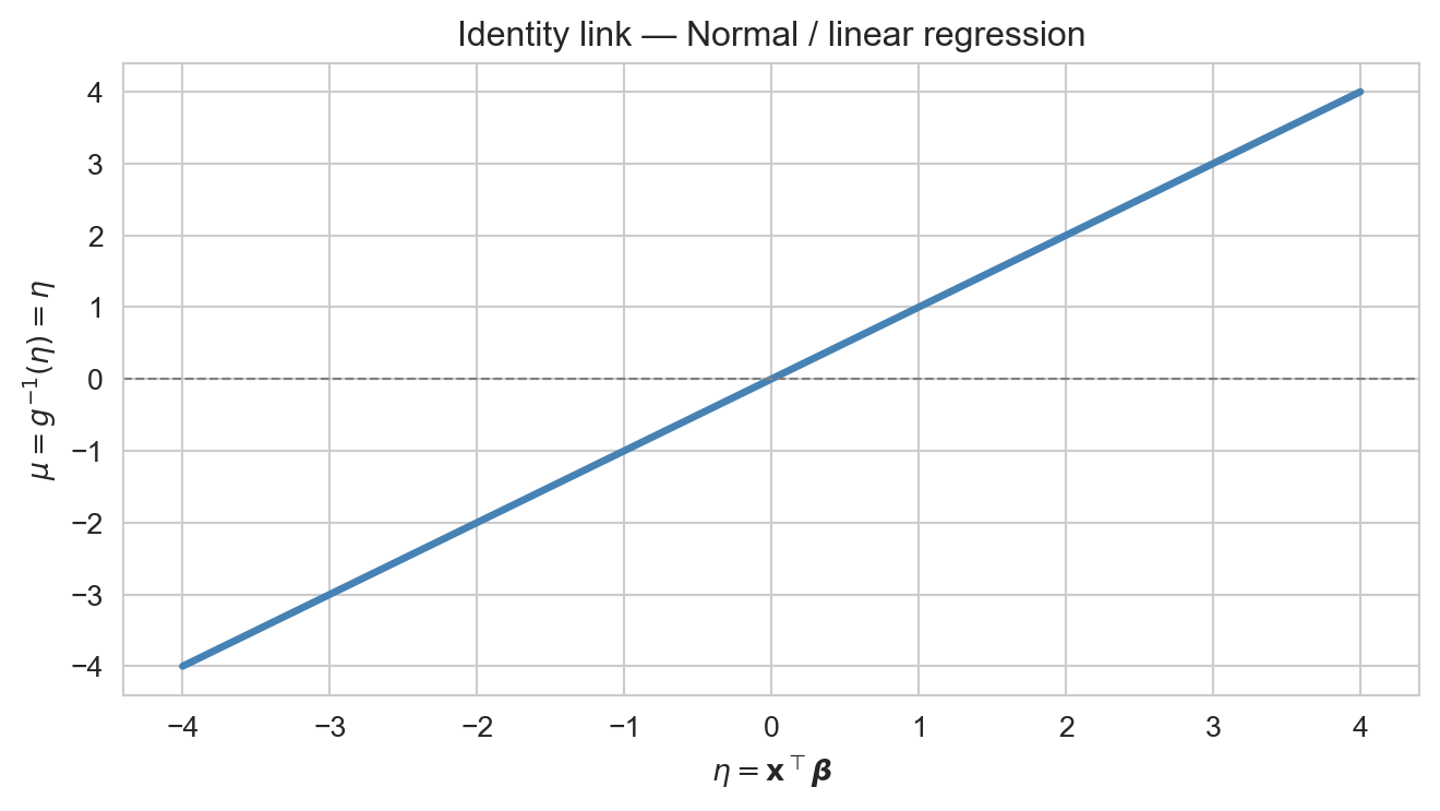
Normal	Continuous \((-\infty, \infty)\)	Identity: \(g(\mu) = \mu\)
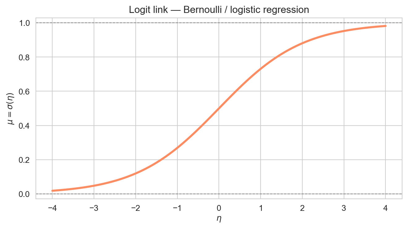
Bernoulli/Binomial	Binary / proportion \([0,1]\)	Logit: \(g(\mu) = \log\frac{\mu}{1-\mu}\)
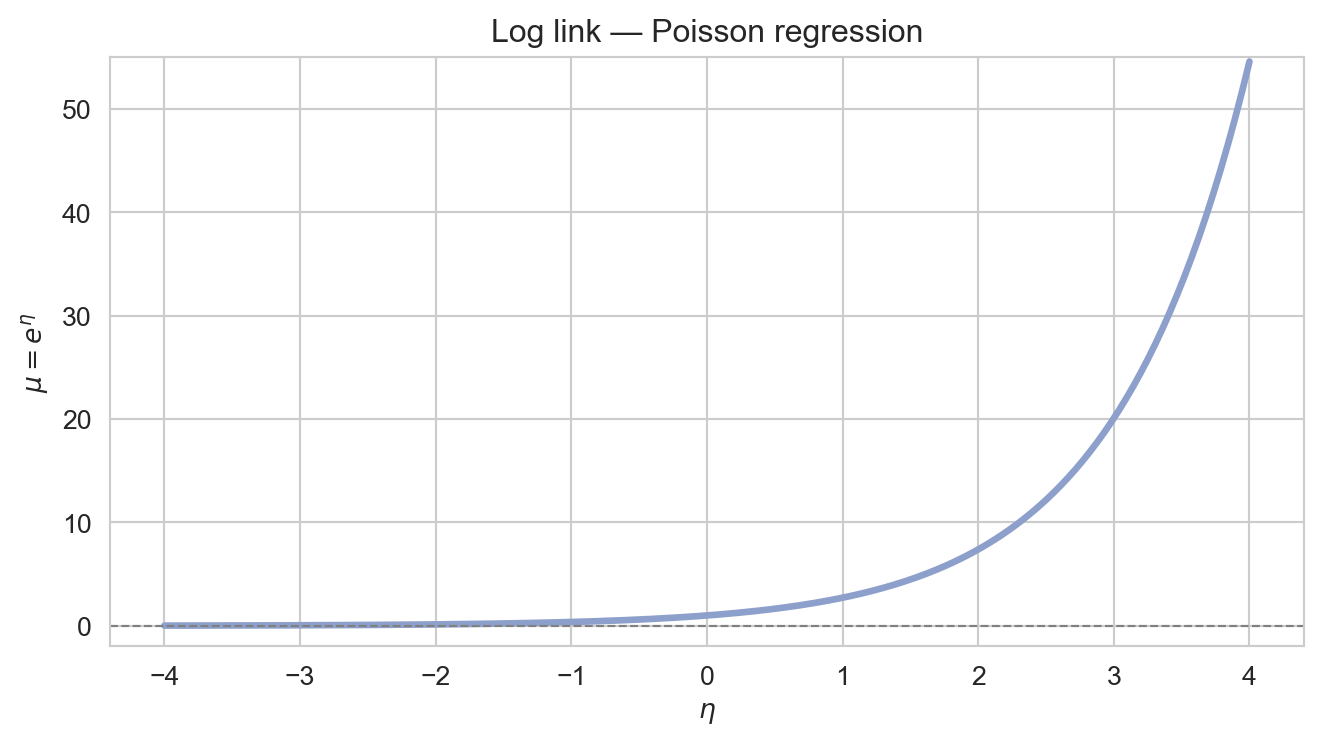
Poisson	Count \(\{0, 1, 2, \ldots\}\)	Log: \(g(\mu) = \log\mu\)
Gamma	Positive continuous \((0, \infty)\)	Inverse: \(g(\mu) = 1/\mu\)

The canonical link is the natural choice derived from the exponential family form and is typically used as a default, though other links can be used if they make scientific sense.

Identity (Normal)

Identity link: \(g(\mu) = \mu\). The mean is modelled directly as the linear predictor, with no constraint — appropriate for continuous, unbounded responses.

Logit (Bernoulli)

Logit link: \(g(\mu) = \log(\mu / (1 - \mu))\). The inverse is the logistic function, which squashes the linear predictor into \((0, 1)\) — appropriate for binary responses.

Log (Poisson)

Log link: \(g(\mu) = \log \mu\). The inverse is the exponential function, which maps the linear predictor to a positive mean — appropriate for count responses.

Estimation: Maximum Likelihood

OLS minimises the sum of squared residuals, which is optimal when errors are Gaussian. For non-Gaussian responses, GLMs are estimated by maximising the log-likelihood:

\[ \ell(\boldsymbol{\beta}) = \sum_{i=1}^n \frac{y_i \theta_i - b(\theta_i)}{a(\phi)} + \text{const}. \]

There is no closed-form solution in general, so we use iteratively reweighted least squares (IRLS). At the current estimate \(\boldsymbol{\beta}^{(t)}\), IRLS computes:

Quantity	Formula	Role
Fitted means	\(\hat{\mu}_i = g^{-1}(\mathbf{x}_i^\top\boldsymbol{\beta}^{(t)})\)	Current predicted means
Weights	\(w_i = 1/\{V(\hat{\mu}_i)[g'(\hat{\mu}_i)]^2\}\)	Downweight noisy observations
Working response	\(z_i = \eta_i + (y_i - \hat{\mu}_i)g'(\hat{\mu}_i)\)	Linearised pseudo-response

It then solves the weighted least squares problem

\[\boldsymbol{\beta}^{(t+1)} = \left(\mathbf{X}^\top \mathbf{W}^{(t)} \mathbf{X}\right)^{-1} \mathbf{X}^\top \mathbf{W}^{(t)} \mathbf{z}^{(t)},\]

repeating until convergence. When applied to the Normal family with the identity link, \(w_i = 1\) for all \(i\) and \(z_i = y_i\) — IRLS reduces to a single step of ordinary least squares. statsmodels handles this automatically.

Deviance and Model Comparison

ImportantDeviance

The deviance of a fitted GLM is: \[D = 2\left[\ell(\text{saturated model}) - \ell(\hat{\boldsymbol{\beta}})\right],\] where the saturated model fits each observation perfectly.

Deviance is the GLM analogue of the residual sum of squares. The null deviance (\(D_0\)) measures fit of the intercept-only model; the residual deviance (\(D\)) measures fit of the fitted model. A large drop \(D_0 - D\) indicates the predictors are useful.

To test whether \(q\) additional parameters significantly improve fit, we use the likelihood ratio test (LRT):

\[G^2 = D_\text{reduced} - D_\text{full} = 2[\ell(\hat{\boldsymbol{\mu}}_\text{full}) - \ell(\hat{\boldsymbol{\mu}}_\text{reduced})] \;\underset{H_0}{\sim}\; \chi^2_q.\]

Reject \(H_0: \beta_{p-q+1} = \cdots = \beta_p = 0\) at level \(\alpha\) if \(G^2 > \chi^2_{q,\,1-\alpha}\). This is the GLM analogue of the partial \(F\)-test; for \(q=1\) it is asymptotically equivalent to the Wald \(z\)-test but preferred in small samples.

References