PSTAT100 Data Science and Analysis

Lecture Notes

Introduction

These are my online lecture notes for the PSTAT100 Data Science and Analysis course taught at UC Santa Barbara. In these lecture notes we study fundamental topics in data science and the tools we use for data retrieval, analysis, visualization, and reproducible research in preparation for advanced data science courses.

Throughout these notes we will conduct our data analysis using python. For information on how to install python as well as a suitable IDE please see my note here. In this section we shall be using the pandas package for data management and the matplotlib package for plotting. Don’t worry if you do not yet understand the code, we shall cover how to perform the analysis in later sections.

import pandas as pd
import matplotlib.pyplot as plt

What is Data Science?

Data science is a nascent field that encompasses a wide range of activities that involve uncovering insights from quantitative information. Data scientists typically combine specific interests (“domain knowledge”, e.g., biology) with computation, mathematics, and statistics and probability to contribute to knowledge in their communities.

Data science involves proceeding through a life cycle. Although the specific steps in this cycle are up for debate, in our course we define them as:

1. Hypothesize: question formulation/refinement.
2. Collect: go out and sample or acquire data ‘second-hand’.
3. Acquaint: get to know your dataset; make friends!
4. Tidy: clean up and organize your data.
5. Explore: search for patterns and structure.
6. Analyze: seek to understand.
7. Interpret: explain the meaning of your analysis.

Data Science Life Cycle (Figure produced by Claude.)

Let’s walk through a simple example to gain an intuition for this cycle by considering the following question:

How do animals’ brains scale with their bodies?

1. Hypothesize

There are lots of datasets out there with brain and body weight measurements, so let’s make the question a bit more specific:

What is the relationship between an animal’s brain and body weight?

It might sound simple, but the relationship is thought to contain clues about evolutionary patterns pertaining to intelligence.

2. Collect

In this case, we won’t directly gather data. Instead, we’ll acquire a publicly available dataset comprising average body weight (kg) and brain weight (g) for 62 mammals.

bb_weights = pd.read_csv('assets/data/mammals.csv').iloc[:, 0:3]
bb_weights.head()

	species	body_weight	brain_weight
0	African elephant	6654.000	5712.0
1	African giant pouched rat	1.000	6.6
2	Arctic fox	3.385	44.5
3	Arctic ground squirrel	0.920	5.7
4	Asian elephant	2547.000	4603.0

3. Acquaint

Since we didn’t collect this data ourselves, we aquaint ourselves with its origins to understand potential limitations. The data was originally collected by Allison and Cicchetti (1976) and only contains mammalian data, no information about birds, fish, reptiles, etc. The species themselves weren’t chosen to represent mammalia hence we probably shouldn’t seek to generalize. Furthermore the values are aggregated data, not individual level.

We conclude that we can only explore the question narrowly for this particular group of animals using the data at hand and have insufficient data to generalize.

4. Tidy

This dataset is already impeccably neat. Each row is an observation for some mammal, and the columns are the two variables (average weight). In this case there is no tidying needed, hence we just check the dimensions and see if any values are missing.

# dimensions?
print("Dimensions: ", "\n", bb_weights.shape)
# missing values?
print("Missingness analysis: ", "\n", bb_weights.isna().sum(axis = 0))

Dimensions:  
 (62, 3)
Missingness analysis:  
 species         0
body_weight     0
brain_weight    0
dtype: int64

5. Explore

Visualization is usually a good starting point. We start by making a simple scatter plot.

fig, ax = plt.subplots()

ax.scatter(bb_weights['body_weight'], bb_weights['brain_weight'],
           color='steelblue', edgecolors='white', linewidths=0.5,
           alpha=0.8, s=60)

ax.set_xlabel('Body weight (kg)')
ax.set_ylabel('Brain weight (g)')
ax.spines[['top', 'right']].set_visible(False)

plt.tight_layout()
plt.show()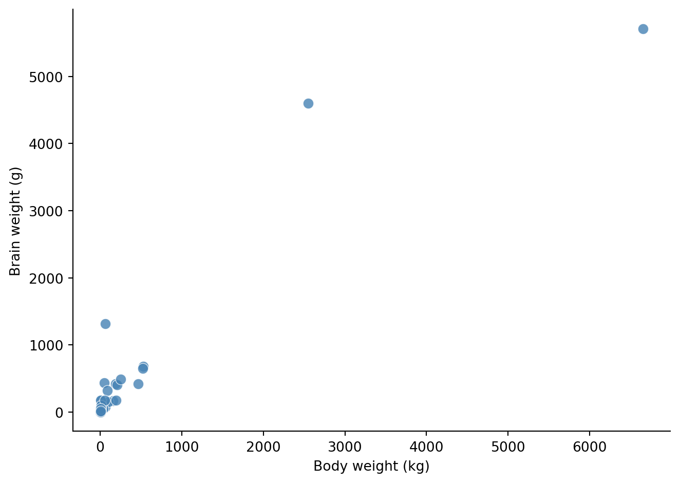

References

Allison, T., and D. V. Cicchetti. 1976. “Sleep in Mammals: Ecological and Constitutional Correlates.” Science 194 (4266): 732–34. https://doi.org/10.1126/science.982039.