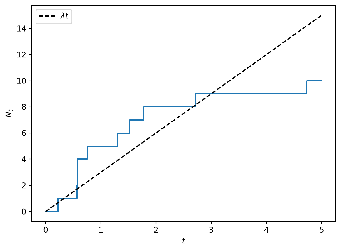
The Poisson process is the canonical continuous-time model for events that occur randomly and independently in time, such as customer arrivals, insurance claims or jumps in an asset price. It is a counting process that increases by one at each event.
A Poisson process with rate \(\lambda>0\) is a process \(\{N_t;t\geq 0\}\) taking values in \(\{0,1,2,\ldots\}\) such that
\(N_0=0\).
Independent increments: for \(0\leq t_0<t_1<\cdots<t_n\) the increments \(N_{t_1}-N_{t_0},\ldots,N_{t_n}-N_{t_{n-1}}\) are independent.
Stationary Poisson increments: for \(s<t\), \[
N_t-N_s\sim\text{Poisson}(\lambda(t-s)).
\]
In particular \(N_t\sim\text{Poisson}(\lambda t)\), so \[
\mathbb{E}[N_t]=\lambda t \quad \& \quad \operatorname{Var}(N_t)=\lambda t,
\] see Poisson Distribution. The parameter \(\lambda\) is the expected number of events per unit time.
2 Infinitesimal Definition
A counting process \(\{N_t\}\) with \(N_0=0\), independent and stationary increments is a Poisson process with rate \(\lambda\) if and only if, as \(h\downarrow 0\), \[
\mathbb{P}(N_{t+h}-N_t=1)=\lambda h+o(h), \quad
\mathbb{P}(N_{t+h}-N_t\geq 2)=o(h).
\]
That is, in a short interval at most one event occurs, with probability proportional to the length of the interval. This is the building block for the birth-death and jump process generalisations.
3 Inter-arrival Times
Let \(T_n=\inf\{t:N_t=n\}\) be the \(n\)-th arrival time and \(\tau_n=T_n-T_{n-1}\) the \(n\)-th inter-arrival time, with \(T_0=0\).
The inter-arrival times \(\tau_1,\tau_2,\ldots\) are i.i.d. \(\text{Exponential}(\lambda)\) random variables. Consequently \[
T_n=\sum_{i=1}^n\tau_i\sim\text{Gamma}(n,\lambda).
\]
Proof. The first arrival occurs after time \(t\) if and only if no events occur in \([0,t]\), so \[
\mathbb{P}(\tau_1>t)=\mathbb{P}(N_t=0)=e^{-\lambda t},
\] which is the survival function of an \(\text{Exponential}(\lambda)\) variable. By independent and stationary increments the process restarts afresh at \(T_1\), so \(\tau_2\) is independent of \(\tau_1\) with the same law, and so on. The sum of \(n\) i.i.d. exponentials is Gamma distributed.
This gives an equivalent definition: a Poisson process is the counting process of a renewal sequence with i.i.d. \(\text{Exponential}(\lambda)\) gaps. The memoryless property of the Exponential Distribution is what makes the process Markov.
4 Conditional Distribution of Arrival Times
Conditional on \(N_t=n\), the arrival times \((T_1,\ldots,T_n)\) have the same distribution as the order statistics of \(n\) i.i.d. \(\text{Uniform}(0,t)\) random variables.
So given the number of events in \([0,t]\), their locations are uniform and independent. This is the basis of the simulation of Poisson processes on a fixed interval: draw \(N_t\sim\text{Poisson}(\lambda t)\), then place \(N_t\) uniform points.
5 Superposition and Thinning
If \(N^{(1)},N^{(2)}\) are independent Poisson processes with rates \(\lambda_1,\lambda_2\), then \(N^{(1)}+N^{(2)}\) is a Poisson process with rate \(\lambda_1+\lambda_2\).
Let \(N\) be a Poisson process with rate \(\lambda\) and mark each event independently as type 1 with probability \(p\) and type 2 with probability \(1-p\). Then the type 1 and type 2 events form independent Poisson processes with rates \(p\lambda\) and \((1-p)\lambda\).
Thinning with a time-dependent retention probability \(p(t)\) is used to simulate the non-homogeneous processes below.
6 Poisson Process as a Markov Chain
\(\{N_t\}\) is a continuous-time Markov Process on \(\mathbb{N}_0\), in fact a pure birth process with constant birth rate \(\lambda_i=\lambda\) and \(\mu_i=0\). Its generator (rate matrix) has entries \[
q_{i,i+1}=\lambda, \quad q_{i,i}=-\lambda, \quad q_{i,j}=0 \text{ otherwise},
\] and the transition probabilities are \[
p_{ij}(t)=\frac{(\lambda t)^{j-i}e^{-\lambda t}}{(j-i)!}, \quad j\geq i.
\]
The Kolmogorov forward equations \(p_{0n}'(t)=\lambda\big(p_{0,n-1}(t)-p_{0n}(t)\big)\) are solved by the Poisson pmf. The process is regular since the holding times \(\text{Exponential}(\lambda)\) sum to infinity, see Jump Process Stability & Regularity.
7 Compensated Poisson Process
The compensated process\(\tilde N_t=N_t-\lambda t\) is a martingale with \[
\mathbb{E}[\tilde N_t]=0, \quad \operatorname{Var}(\tilde N_t)=\lambda t,
\] and so is \(\tilde N_t^2-\lambda t\).
Proof. For \(s<t\), by independent increments \[
\mathbb{E}[N_t-\lambda t\mid\mathcal{F}_s]
=N_s+\lambda(t-s)-\lambda t=N_s-\lambda s.
\]
8 Generalisations
Non-homogeneous Poisson process. The rate is a deterministic function \(\lambda(t)\) and \[
N_t-N_s\sim\text{Poisson}\left(\int_s^t\lambda(u)\,du\right).
\] Increments remain independent but are no longer stationary.
Compound Poisson process. Each event carries an i.i.d. jump size \(Y_i\), \[
X_t=\sum_{i=1}^{N_t}Y_i,
\] see Compound Poisson Distribution. This is the simplest Lévy jump process and is used for insurance claims and jump-diffusion models.
Cox (doubly stochastic) process. The rate \(\lambda_t\) is itself a random process, giving over-dispersion (\(\operatorname{Var}(N_t)>\mathbb{E}[N_t]\)).
9 Simulation
Using the inter-arrival representation:
import numpy as npimport matplotlib.pyplot as pltrng = np.random.default_rng(0)lam, T =3.0, 5.0# Exponential gaps until time T is exceededgaps = rng.exponential(1/ lam, size=int(5* lam * T))arrivals = np.cumsum(gaps)arrivals = arrivals[arrivals <= T]plt.step(np.r_[0, arrivals, T], np.r_[0, np.arange(1, len(arrivals) +1),len(arrivals)], where="post")plt.plot([0, T], [0, lam * T], "k--", label=r"$\lambda t$")plt.xlabel("$t$")plt.ylabel("$N_t$")plt.legend()plt.show()