Gaussian Integral
Gaussian Integral
In Probability Theory the Normal Distribution is a continuous probability distribution with parameters mean \(\mu\) and variance \(\sigma^2\) that takes the form of a bell-shaped curve that is symmetric about the mean. For a Normal random variable \(X\sim\mathcal{N}(\mu,\sigma^2)\) can take values in \(\mathbb{R}\) and has probability density function (PDF) of the normal distribution is given by
\[ f(x;\mu,\sigma^2)=\frac{1}{\sqrt{2\pi\sigma^2}} \exp\left(-\frac{(x-\mu)^2}{2\sigma^2}\right). \]
Now, since this is a probability distribution, we know that the total probability must be equal to 1, that is
\[ \int_{-\infty}^{\infty} \frac{1}{\sqrt{2\pi\sigma^2}} \exp\left(-\frac{(x-\mu)^2}{2\sigma^2}\right) dx = 1. \]
The purpose of this note is to demonstrate how to compute this integral analytically.
Standard Normal
First lets evaluate the following Gaussian integral
\[ I = \int_{-\infty}^{\infty} \exp\left(-\frac{x^2}{2}\right) dx. \]
Since the integrand is non-negative, Tonelli’s theorem allows us to square the integral as
\[ I^2 = \int_{-\infty}^{\infty} \exp\left(-\frac{x^2}{2}\right) dx \int_{-\infty}^{\infty} \exp\left(-\frac{y^2}{2}\right) dy = \int_{-\infty}^{\infty} \int_{-\infty}^{\infty} \exp\left(-\frac{x^2+y^2}{2}\right) dx dy. \]
We can then change to polar coordinates
\[ y = r\sin(\theta), \quad x = r\cos(\theta), \quad r\in [0,\infty), \theta\in[0,2\pi). \]
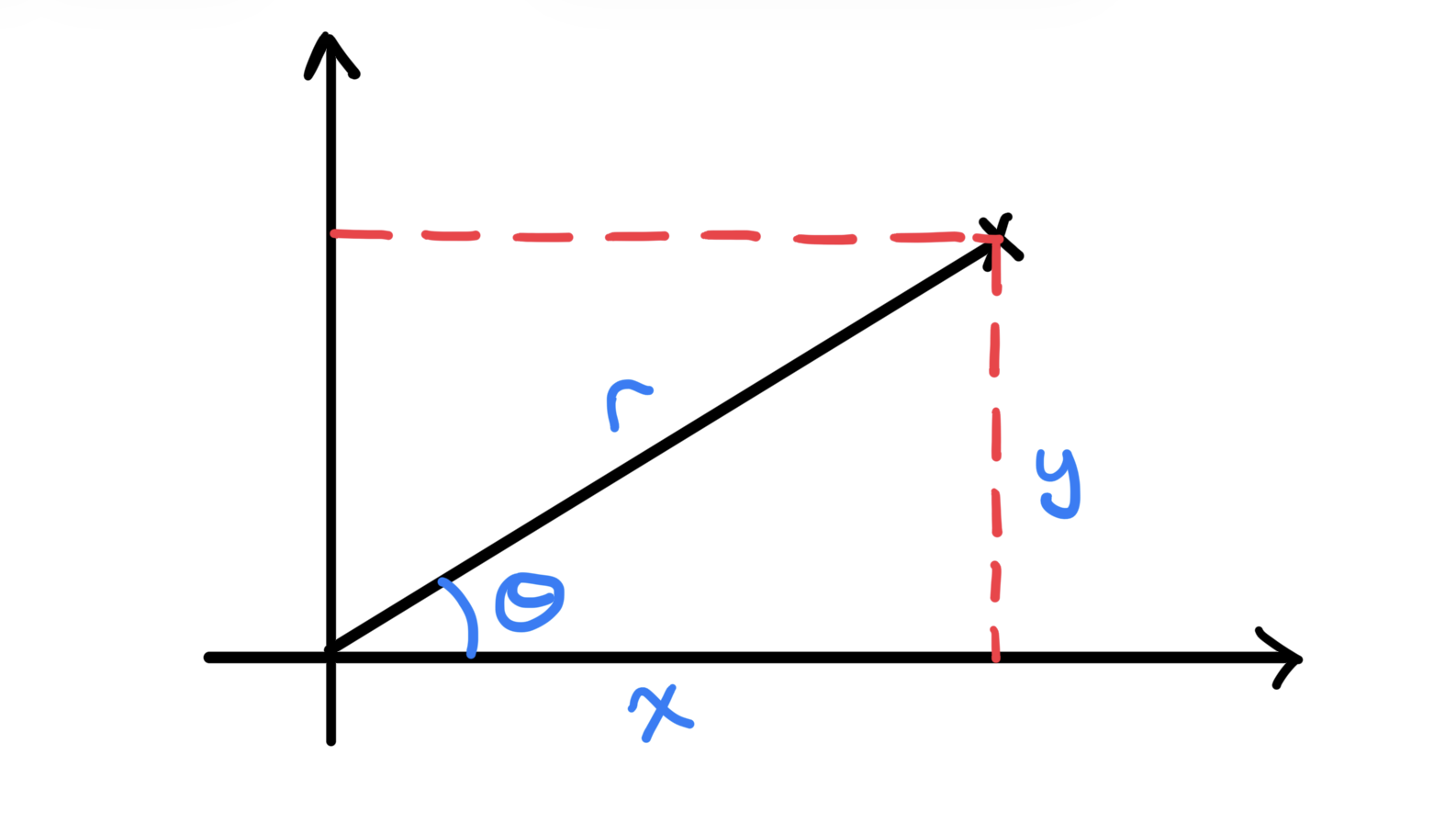
The Jacobian Matrix of the transformation is given by
\[ \begin{align} J & = \lvert \frac{\partial (x,y) }{\partial (r,\theta)}\rvert| = \left\lvert \begin{matrix} \frac{\partial x}{\partial r} & \frac{\partial x}{\partial \theta} \\ \frac{\partial y}{\partial r} & \frac{\partial y}{\partial \theta} \end{matrix} \right\rvert = \left\lvert \begin{matrix} \cos(\theta) & -r\sin(\theta) \\ \sin(\theta) & r\cos(\theta) \end{matrix} \right\rvert \\ & = r \cos^2(\theta) + r\sin^2(\theta)= r. \end{align} \]