Lecture 5: Data Visualization

PSTAT100: Data Science - Concepts and Analysis

John Inston

johninston@ucsb.edu

University of California, Santa Barbara

May 6, 2026

🚁 Overview

Aims of the lecture

Introduce the concept of data visualization and its importance in data analysis.
Provide an overview of basic visualizations and when to use them.
Introduce the matplotlib and seaborn libraries for creating visualizations in Python.
Explore various style and formatting features including:
- Themes.
- Variable Formatting
- Facets.

📚 Required Libraries

In this lecture we will be using the following libraries:

import pandas as pd
import numpy as np
import matplotlib.pyplot as plt
import seaborn as sns

Recap: Data Preparation

Data Preparation

So far we have covered:
- Data acquisition and understanding.
- Data preparation.
  - Tidy data.
  - Quality assessment.
  - Data cleaning.

Next Step: Exploration

Perform exploratory data analysis (EDA).
Learn data properties and relationships.

Exploratory Data Analysis (EDA)

🔍 Exploratory Data Analysis (EDA)

What is EDA?

Exploratory Data Analysis (EDA)

Exploratory Data Analysis (EDA) is the process of analyzing and visualizing data to understand its structure, identify patterns, and uncover insights.

EDA Steps (Topic of next lecture)

Perform univariate analysis to understand the distribution of individual variables.
Perform multivariate analysis to explore relationships between variables.
Develop insights to inform modeling and deeper analysis.

Data Visualization

A key component of EDA is data visualization.
Python’s standard library does not include a full visualization system, so we use dedicated libraries such as:
- matplotlib, seaborn, altair, and plotly.

Data Visualization

Why Visualize Data?

Improve interpretability of data.
Identify patterns and relationships.
Communicate findings effectively.
Explore data in an interactive way.

Principles of Effective Data Visualization

Novel
Informative
Efficient
Aesthetic

Always ask yourself, what is this visualization for? What is it contributing?

Types of Visualization

Exploratory vs Presentation

Exploratory visualizations
- Used during the data analysis process to explore and understand the data.
- Often created quickly and may not be polished or refined.
Presentation visualizations
- Used to communicate findings to an audience.
- Typically more polished and refined, with a focus on clarity and aesthetics.

Static vs Interactive vs Animated

Static visualizations: These are fixed images that do not allow for user interaction.
Interactive visualizations: These allow users to interact with the data, such as zooming, filtering, and hovering for more information.
Animated visualizations: These show changes in data over time or through different conditions.

Visualizations in Python

`matplotlib`

The foundational visualization library in Python.
Almost every other Python visualization library — including seaborn — is built on top of it.
It is an imperative visualization library, meaning:
- Total control over all plot details.
- Often more verbose for common plots.
Strong for fine-grained customization and publication-style figures.

`seaborn`

Declarative statistical visualization library for Python.
- Similar to ggplot2 in R.

It is a high-level statistical plotting API on top of matplotlib, meaning:
- You can create common statistical visualizations with much less code.
- It provides useful defaults for themes, color palettes, and grouped comparisons.
Well suited for EDA and rapid iteration.

`altair`

A declarative statistical visualization library for Python, based on Vega and Vega-Lite.
It allows you to create interactive visualizations with a simple and intuitive syntax.
Good for EDA, interactive documents, and reproducible chart specifications.

Plan for upcoming lectures

Lecture 5 (Today)

Summary of standard visualizations and when to use them.
- Univariate, bivariate, multivariate.
- Categorical vs continuous variables.
Outline standard basic (static) visualization production.
- Summarize foundations in matplotlib.
- Focus on seaborn for EDA visualizations.

Lecture 6 (Thursday)

Exploratory Data Analysis (EDA).
Descriptive statistics.
Complex seaborn visualizations.
Interactive visualizations with altair.

Basic Visualizations

Standard Visualizations

We use different plots to visualize different types of data and relationships.
- Univariate and continuous variables:
  - Box plots, Violin plots:
    - Visualize the descriptive statistics of a continuous variable.
  - Histograms, Density plots
    - Visualize the distribution of a continuous variable.
- Univariate and categorical variables:
  - Bar plots, Count plots
    - Visualize the count or proportion of categories in a categorical variable.
- Bivariate and continuous:
  - Scatter plots
    - Visualize the relationship between two continuous variables.
  - Line plots
    - Visualize the relationship between two continuous variables over time or another continuous dimension.

Example Data: `penguins`

We will be using the penguins dataset loaded from the seaborn library.
Contains measurements of penguins from three different species: Adelie, Chinstrap, and Gentoo.

penguins = sns.load_dataset("penguins")
print(penguins.shape)
penguins.head()

(344, 7)

	species	island	bill_length_mm	bill_depth_mm	flipper_length_mm	body_mass_g	sex
0	Adelie	Torgersen	39.1	18.7	181.0	3750.0	Male
1	Adelie	Torgersen	39.5	17.4	186.0	3800.0	Female
2	Adelie	Torgersen	40.3	18.0	195.0	3250.0	Female
3	Adelie	Torgersen	NaN	NaN	NaN	NaN	NaN
4	Adelie	Torgersen	36.7	19.3	193.0	3450.0	Female

Object-Oriented Interface

Pyplot vs Object-Oriented Interface

Pyplot interface: A state-based interface that allows you to create plots using a simple, MATLAB-like syntax. It is suitable for quick and simple visualizations.
Object-oriented interface: A more flexible and powerful interface that allows you to create complex and customized plots by working with figure and axes objects directly. It is recommended for more complex visualizations and when you need more control over the plot.
- We will primarily be using the object-oriented interface in this course.

Only covering the basics of `matplotlib`

We will focus on plotting in seaborn and altair in this course.
We only cover what we need to know in matplotlib.

`matplotlib` Scatter Plots

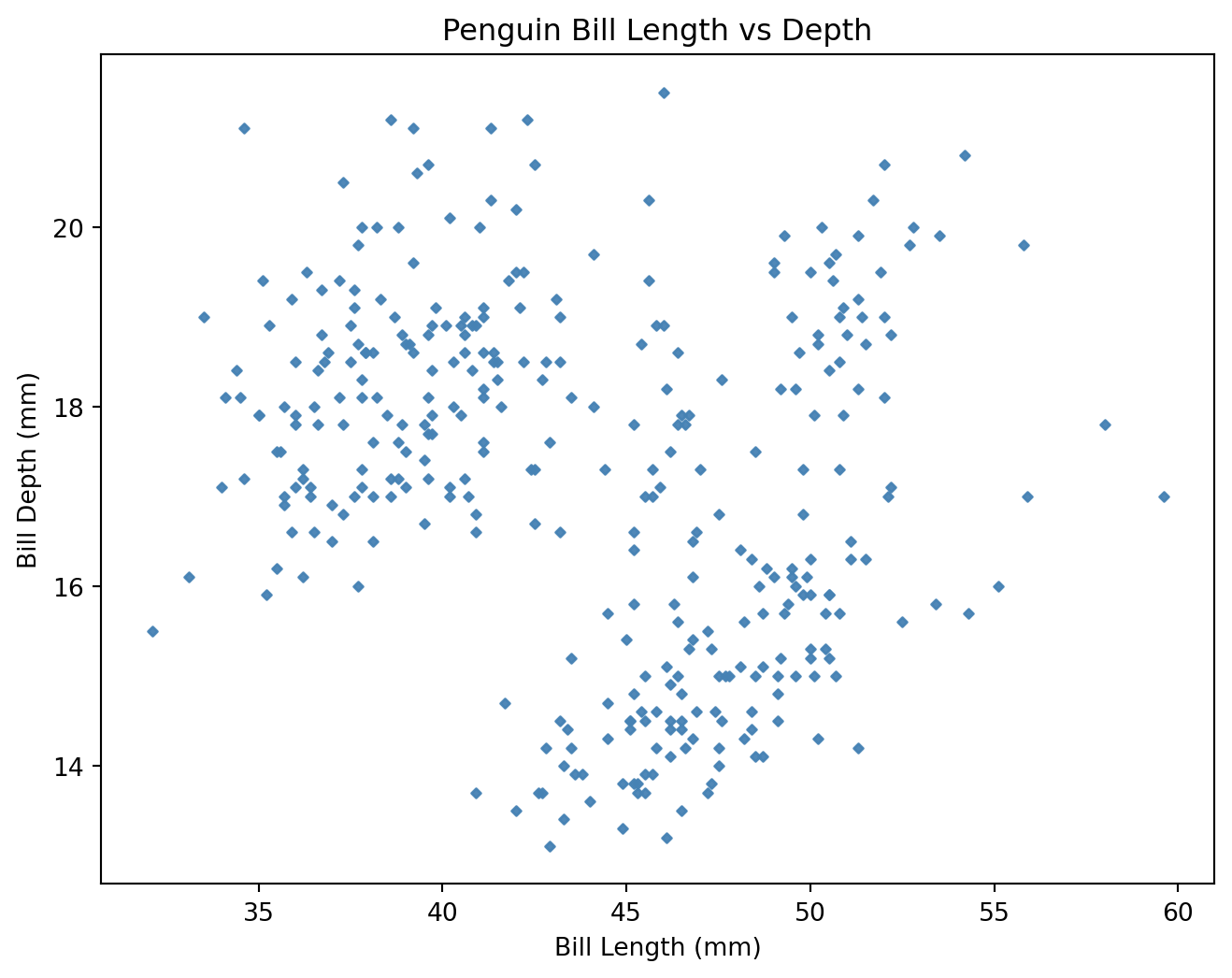
Scatter Plots

A scatter plot pairs two continuous variables to visualize their relationship.
We produce scatter plots in matplotlib as follows:
- Create a figure and axis object using plt.subplots().
- Call the appropriate plotting function on the axis object (e.g. ax.scatter()).
- Customize the plot using axis methods ax.set().
- Display the plot using plt.show().

fig, ax = plt.subplots(figsize=(8, 6))          # Create figure and axis objects
ax.scatter (                                    # Create scatter plot
    "bill_length_mm", "bill_depth_mm",       
    data=penguins,                      
    color="steelblue",                          # Set point color
    alpha=0.95,                                 # Set point transparency
    s=7,                                        # Set point size
    marker="D"                                  # Set point type
    )
ax.set(                                         # Set labels and title
  xlabel="Bill Length (mm)",
  ylabel="Bill Depth (mm)",
  title="Penguin Bill Length vs Depth"
)
plt.show()                                     # Show the plot

`matplotlib` Scatter Plots

Scatter plot of bill length vs bill depth for the penguins dataset. (`matplotlib`)

`seaborn` Scatter Plots

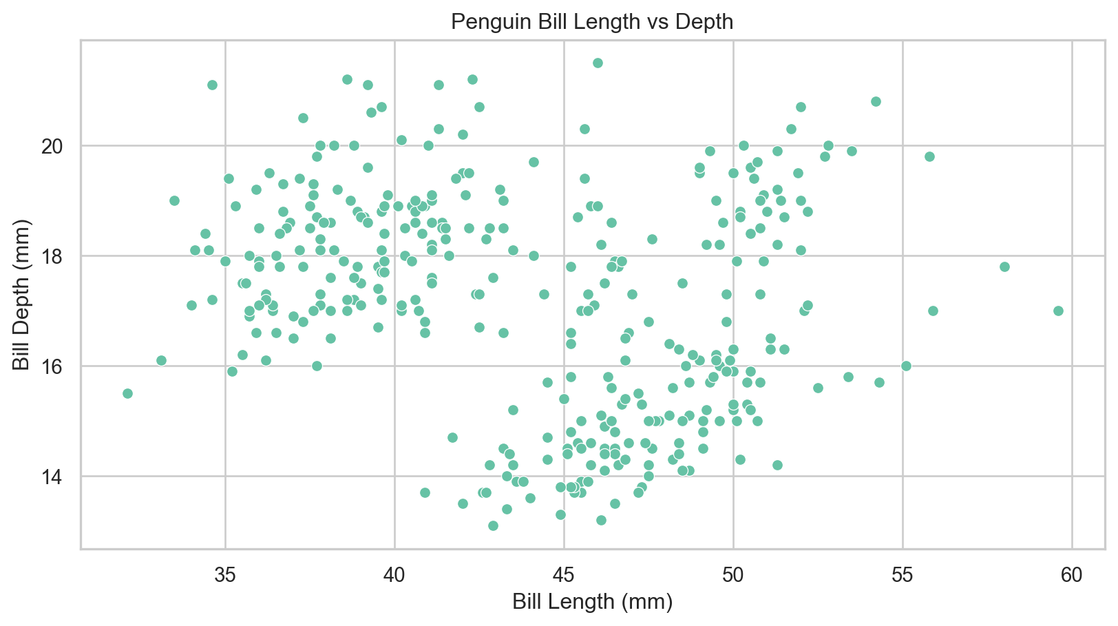
What makes `seaborn` so great?

Uses the same underlying plotting functions as matplotlib but provides a higher-level interface for creating more complex and informative visualizations with less code.
Provides built-in themes and color palettes to make it easy to create attractive visualizations.
Provides functions for visualizing statistical relationships, such as regression lines and confidence intervals.

Scatter Plots in `seaborn`

sns.set_theme(style="whitegrid", palette="Set2")             # Set theme
ax = sns.scatterplot(                             # Create scatter plot
    x="bill_length_mm", y="bill_depth_mm",  
    data=penguins
)
ax.set(
  xlabel="Bill Length (mm)", 
  ylabel="Bill Depth (mm)", 
  title="Penguin Bill Length vs Depth")
plt.show()                                   # Show the plot

`seaborn` Scatter Plots

Scatter plot of bill length vs bill depth for the penguins dataset. (`seaborn`)

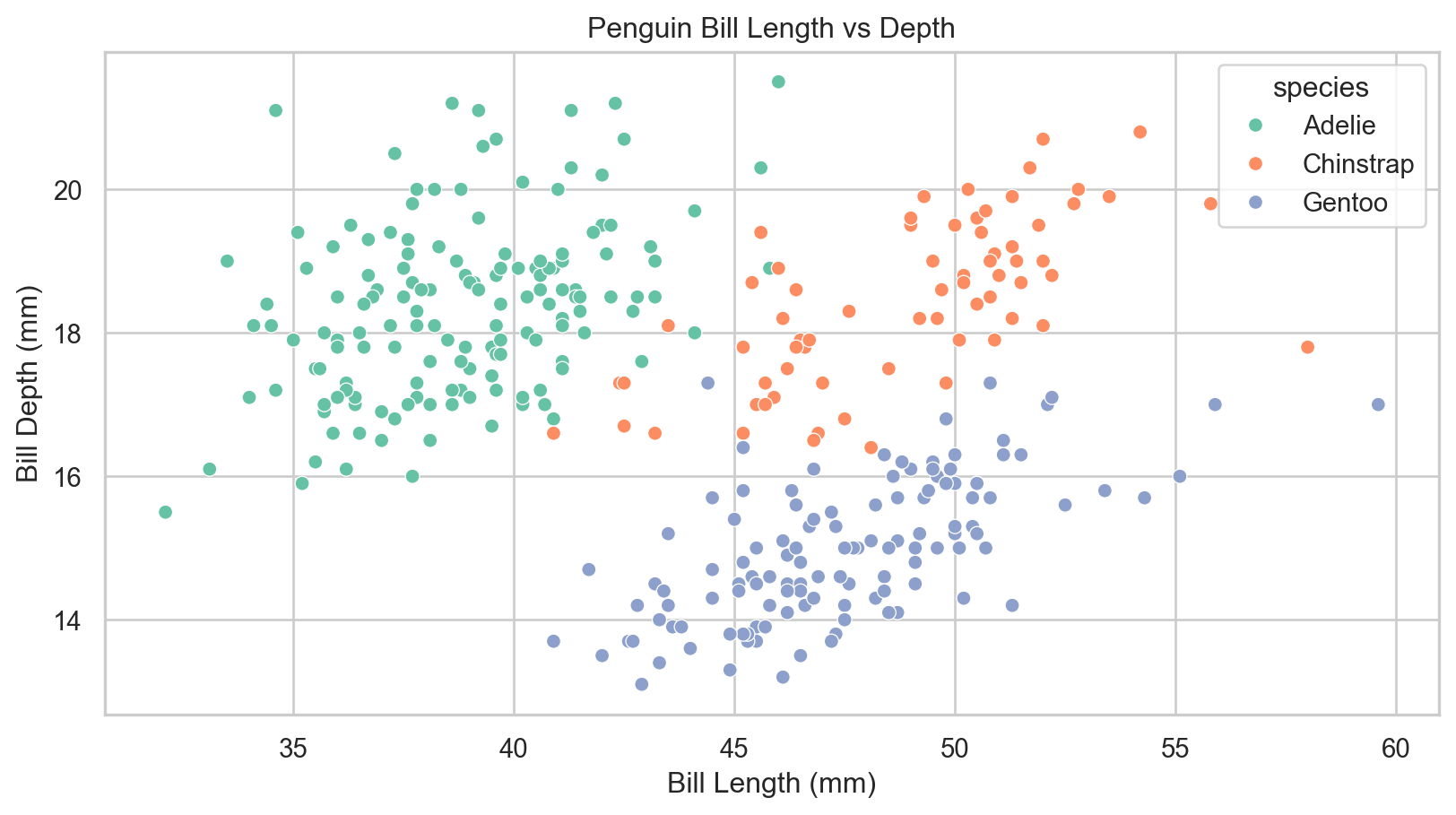
Variable Based Formatting

Often we would like to examine the influence of a third categorical variable on the relationship between two continuous variables.
We can use variable-based formatting to color points by species in the penguins dataset.

Scatter Plots with Variable Based Formatting in `seaborn`

ax = sns.scatterplot(                             
    x="bill_length_mm", y="bill_depth_mm",  
    data=penguins,
    hue="species"                           # Color points by species
)
ax.set(
  xlabel="Bill Length (mm)", 
  ylabel="Bill Depth (mm)", 
  title="Penguin Bill Length vs Depth")
plt.show()

Variable Based Formatting

Scatter plot of bill length vs bill depth grouped by species for the penguins dataset. (`seaborn`)

Adding Best Fit Lines

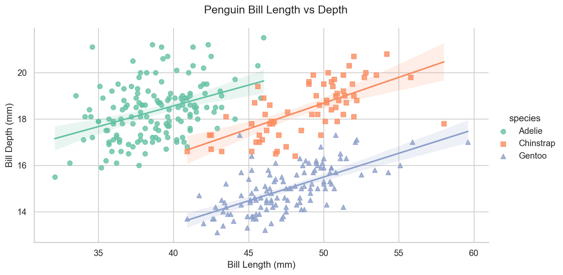
What are best fit lines?

A best fit line is a line that best fits the data points in a scatter plot, showing the overall trend of the relationship between the two variables.
In seaborn, we can produce a scatter plot with a best fit line using the lmplot() function.

For now, treat best fit lines as descriptive trend summaries; we will cover regression assumptions, estimation, and interpretation in detail in future weeks.

`seaborn` Regression Lines

g = sns.lmplot(                               # Scatter with regression line
    x="bill_length_mm", y="bill_depth_mm",  
    data=penguins,
    hue="species",                                      
    markers=["o", "s", "^"],                # Set point types
    line_kws={"linewidth": 2},               # Set line width
    height=5, aspect=1.8                    # Change figure size
)
g.set_axis_labels("Bill Length (mm)", "Bill Depth (mm)")
g.fig.subplots_adjust(top=0.9)
g.fig.suptitle("Penguin Bill Length vs Depth")
plt.show()

Adding Best Fit Lines

Scatter plot of bill length vs bill depth grouped by species with best fit lines and confidence intervals for the penguins dataset. (`seaborn`)

Bar Plots

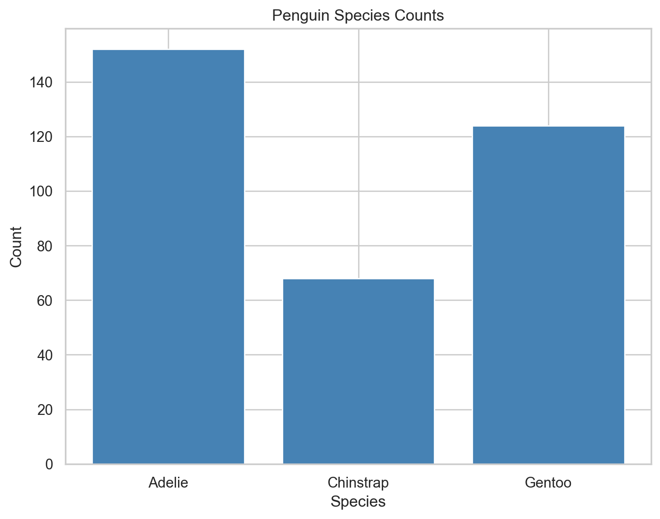
What are bar plots?

A bar plot is a chart that presents categorical data with rectangular bars, where the length of each bar is proportional to the value it represents.
They are often used to represent the count or proportion of categories in a categorical variable.
Bar plots in matplotlib are driven by the summary data frame we provide. In this case, we compute species counts in advance.

`matplotlib` Bar Plots

bp1_data = penguins.groupby("species").size(
  ).reset_index(name="count")
print(bp1_data)

     species  count
0     Adelie    152
1  Chinstrap     68
2     Gentoo    124

fig, ax = plt.subplots(figsize=(8, 6))
ax.bar(
  x="species", 
  height="count", 
  data=bp1_data, 
  color="steelblue"
  )
ax.set(
  xlabel="Species", 
  ylabel="Count", 
  title="Penguin Species Counts")
plt.show()

Bar Plots

Bar plot of penguin species counts for the penguins dataset. (`matplotlib`)

Count Plots

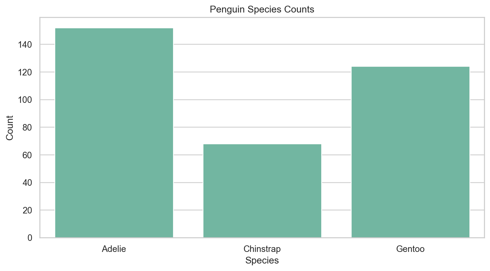
`seaborn` Count Plots

Although seaborn has an equivalent barplot function, a more useful plot type in this case is a countplot.
This automatically computes the counts for each category and creates a bar plot without needing to pre-aggregate the data.

ax = sns.countplot(
    x="species",
    data=penguins
)
ax.set(
  xlabel="Species", 
  ylabel="Count", 
  title="Penguin Species Counts")
plt.show()

Count Plots

Bar plot of penguin species counts for the penguins dataset. (`seaborn`)

Subgrouping and Variable Formatting

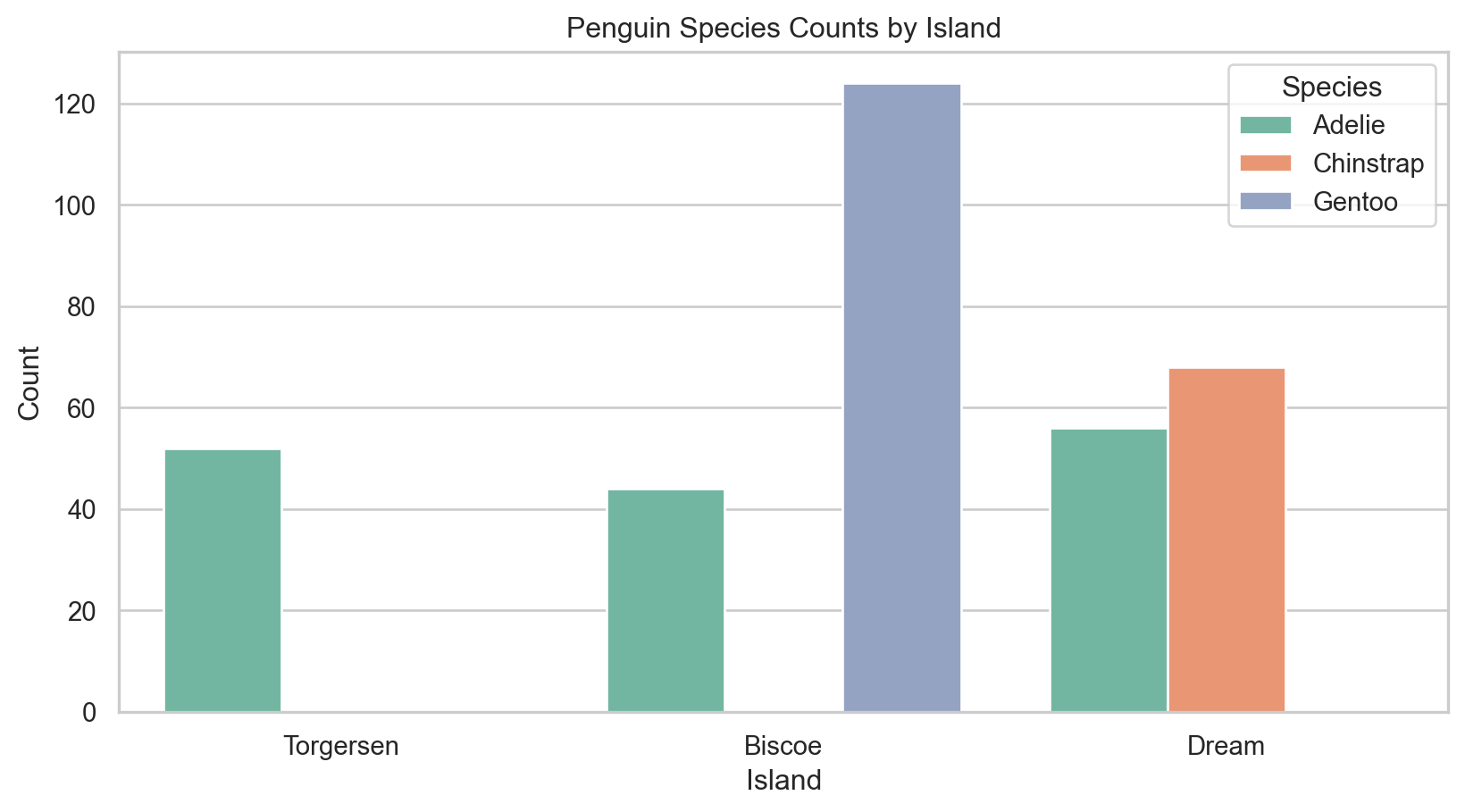
Subgrouping

To examine relationships between multiple categorical variables, we can split each bar into subgroups based on a second categorical variable (e.g., species and island).

Subgrouped Bar Plot with Variable Formatting

ax = sns.countplot(
    x="island",
    hue="species",
    data=penguins
)
ax.set(
  xlabel="Island", 
  ylabel="Count", 
  title="Penguin Species Counts by Island"
  )
ax.legend(title="Species")
plt.show()

Subgrouping and Variable Formatting

Box Plots

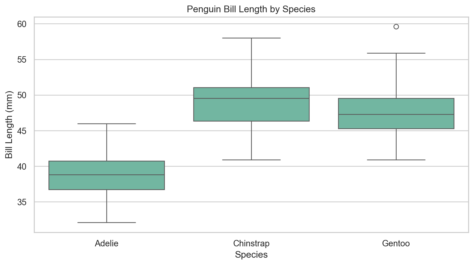
What are box plots?

A box plot (or box-and-whisker plot) is a standardized way of displaying the distribution of data based on a five-number summary: minimum, first quartile (Q1), median, third quartile (Q3), and maximum.
It can also show outliers in the data.
In seaborn, we can produce a box plot using the boxplot() function.

`seaborn` Box Plots

ax = sns.boxplot(
    x="species", y="bill_length_mm",
    data=penguins
)
ax.set(
  xlabel="Species", 
  ylabel="Bill Length (mm)", 
  title="Penguin Bill Length by Species"
  )
plt.show()

Box Plots

Box plot of bill length by species for the penguins dataset. (`seaborn`)

Histograms

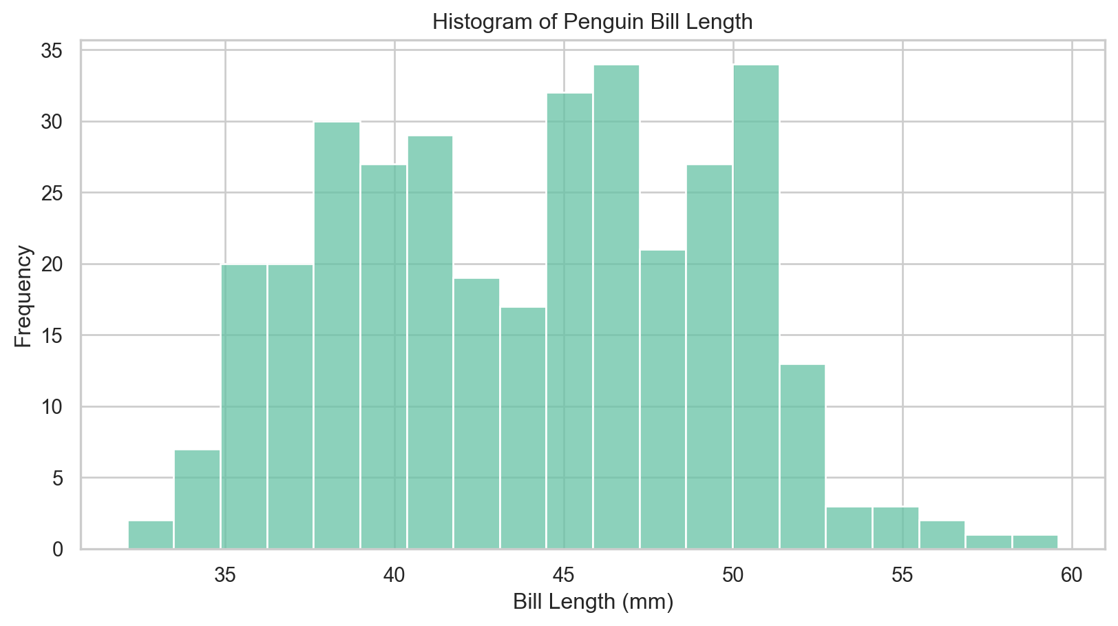
What are histograms?

A histogram is a graphical representation of the distribution of a dataset, where the data is divided into bins and the frequency of data points in each bin is represented by the height of the bar.
In seaborn, we can produce a histogram using the histplot() function.

`seaborn` Histograms

ax = sns.histplot(
    x="bill_length_mm",
    data=penguins,
    bins=20                 # Set number of bins
)
ax.set(xlabel="Bill Length (mm)", ylabel="Frequency", title="Histogram of Penguin Bill Length")
plt.show()

Histograms

Histogram of bill length for the penguins dataset. (`seaborn`)

Histograms with Variable Formatting and Kernel Density Estimates

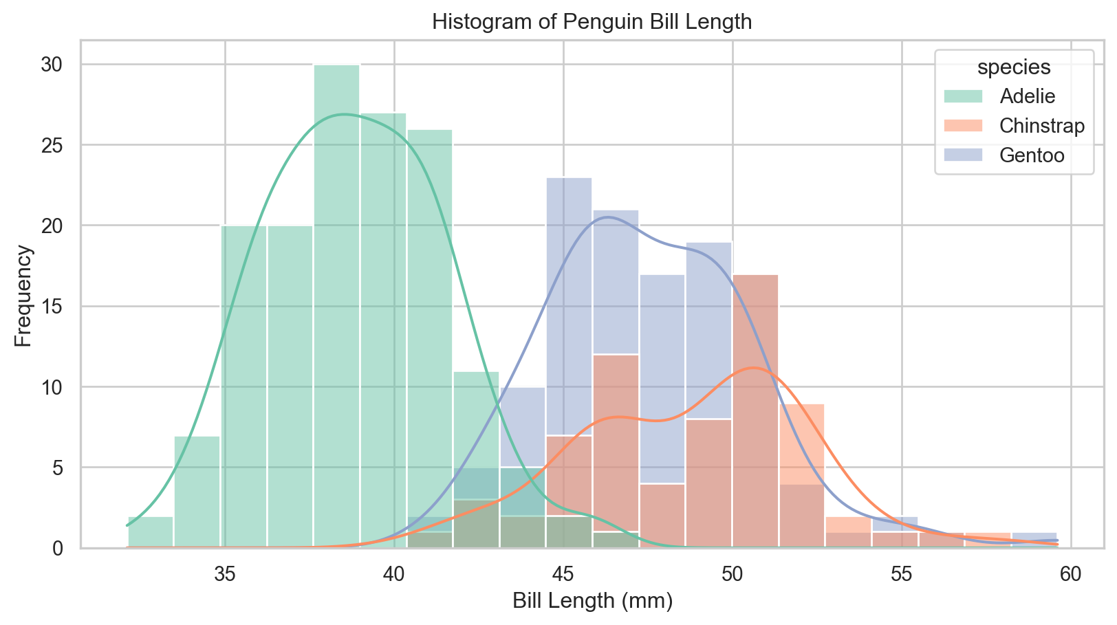
Let’s start exploring what we can do!

We know that the three species of penguins have different bill length distributions.
- Can we visualize this in a single plot?
We can produce kernel density estimates (KDEs) to visualize the distribution of bill length for each species in a single plot.

`seaborn` Histograms with KDEs

Histogram shape depends on binning choices, and KDE smoothness depends on bandwidth, so use these as exploratory summaries rather than definitive evidence.

ax = sns.histplot(
    x="bill_length_mm",
    data=penguins,
    bins=20,                # Set number of bins
    kde=True,               # Show kernel density estimate
    hue="species",          # Color by species
    multiple="layer"        # Overlay histograms
)
ax.set(xlabel="Bill Length (mm)", ylabel="Frequency", title="Histogram of Penguin Bill Length")
plt.show()

Histograms with Variable Formatting and Kernel Density Estimates

Violin Plots

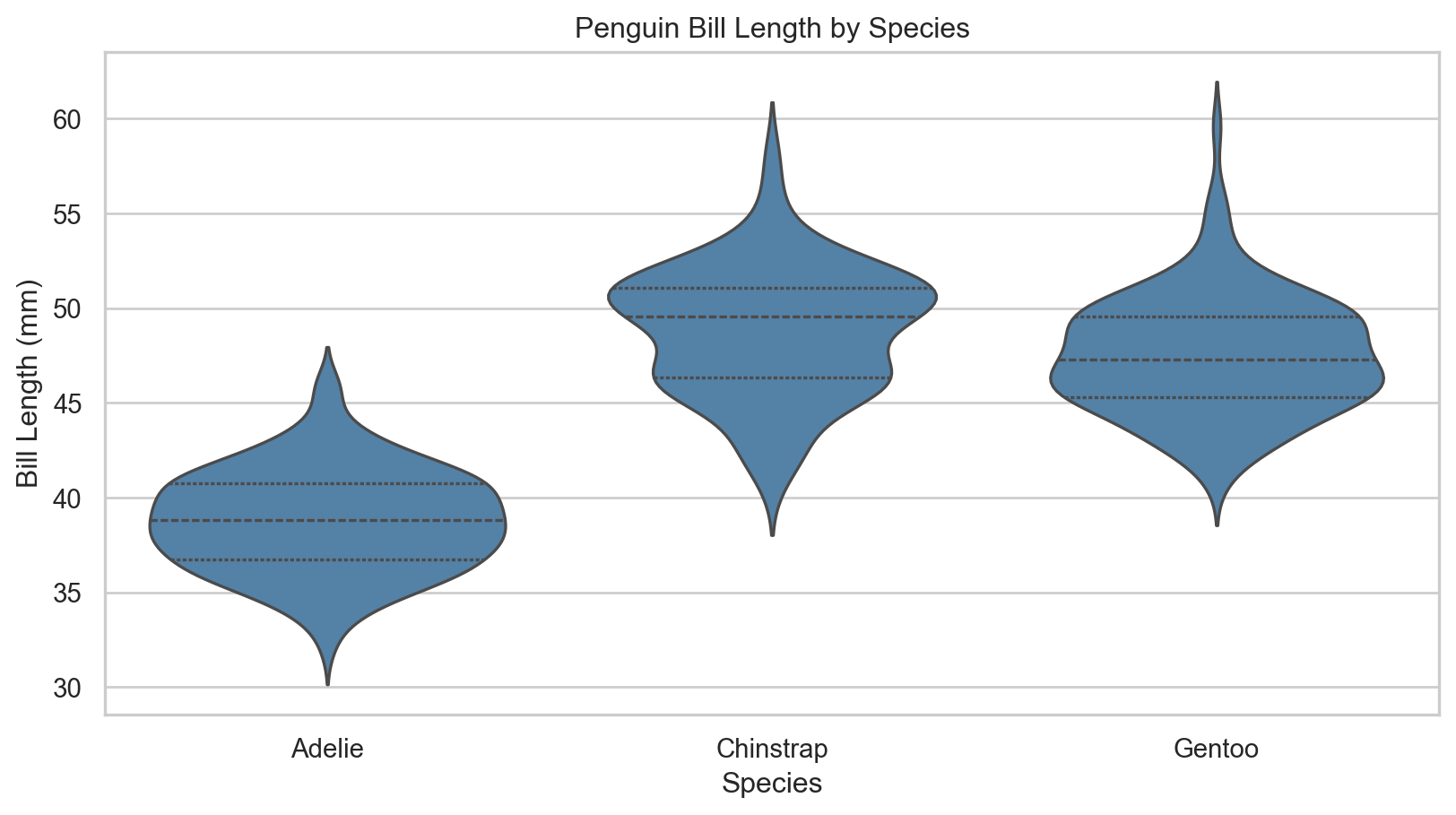
Fancy box plots?

A violin plot is a method of plotting numeric data and can be understood as a combination of a box plot and a kernel density plot (a smoothed version of a histogram).
It provides a visual summary of the distribution of the data, including its central tendency, variability, and shape.
In seaborn, we can produce a violin plot using the violinplot() function.

Violin Plots in `seaborn`

ax = sns.violinplot(
    x="species", y="bill_length_mm",
    data=penguins,
    inner="quartile",              # Show quartiles inside the violin
    color="steelblue"        # Set violin color
)
ax.set(
  xlabel="Species", 
  ylabel="Bill Length (mm)", 
  title="Penguin Bill Length by Species"
  )
plt.show()

Violin Plots

Violin plot of bill length by species for the penguins dataset. (`seaborn`)

Advanced Visualizations

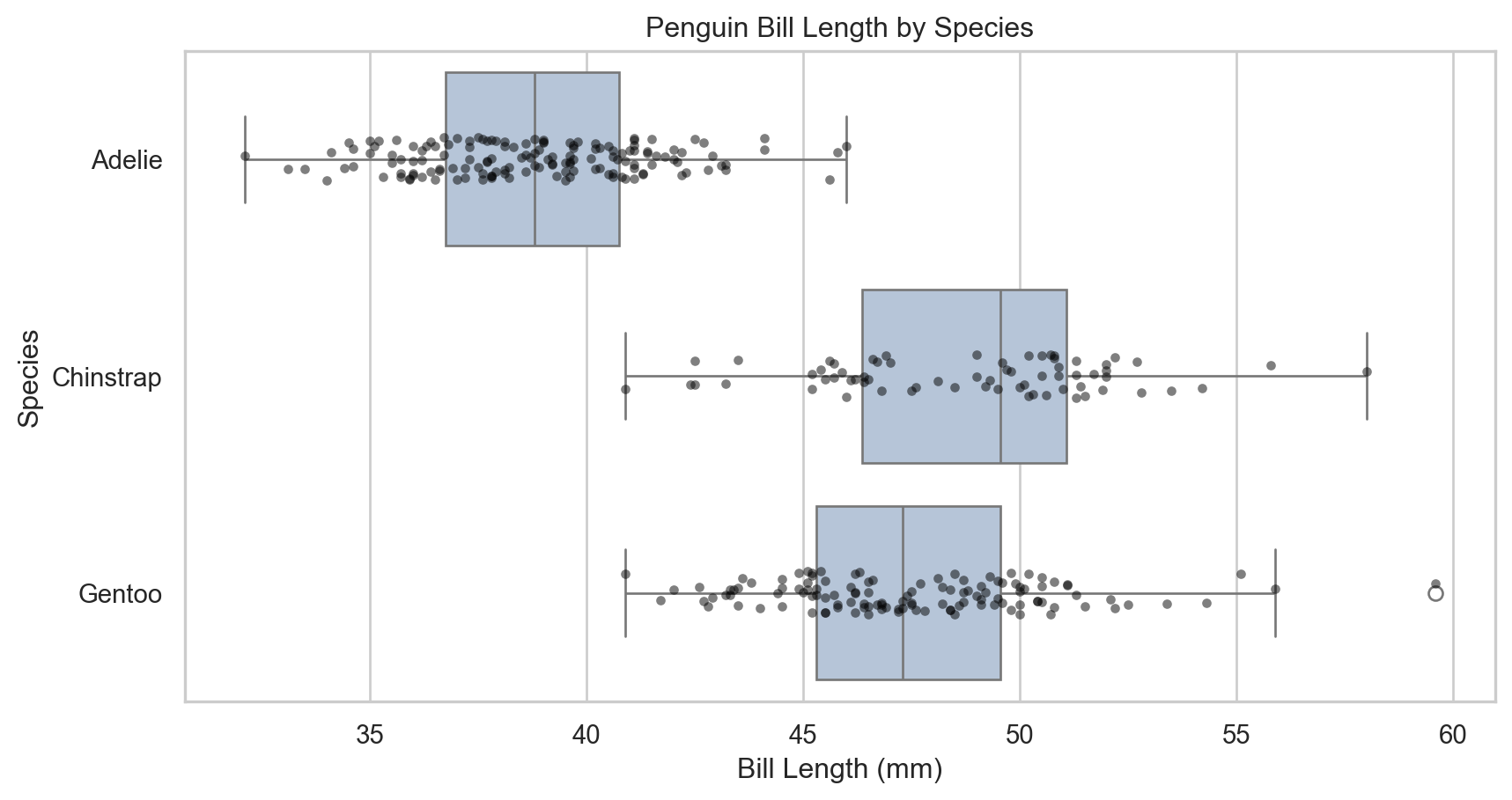
Be creative!

Remember, the goal of visualization is to communicate in a novel, aesthetic, and informative way.
Don’t be afraid to experiment with different visualizations.
Tweak and change things until they are clear!

Perhaps this boxplot is more informative?

ax = sns.boxplot(
    x="bill_length_mm", y="species",
    data=penguins,
    color="lightsteelblue"
)
sns.stripplot(
    x="bill_length_mm", y="species",
    data=penguins,
    color="black",         # Use a single point color for readability
    alpha=0.5,           # Set point transparency
    size=4,              # Set point size
    ax=ax
)
ax.set(
  xlabel="Bill Length (mm)", 
  ylabel="Species", 
  title="Penguin Bill Length by Species"
  )
plt.show()

Advanced Visualizations

Continuous Variable Formatting

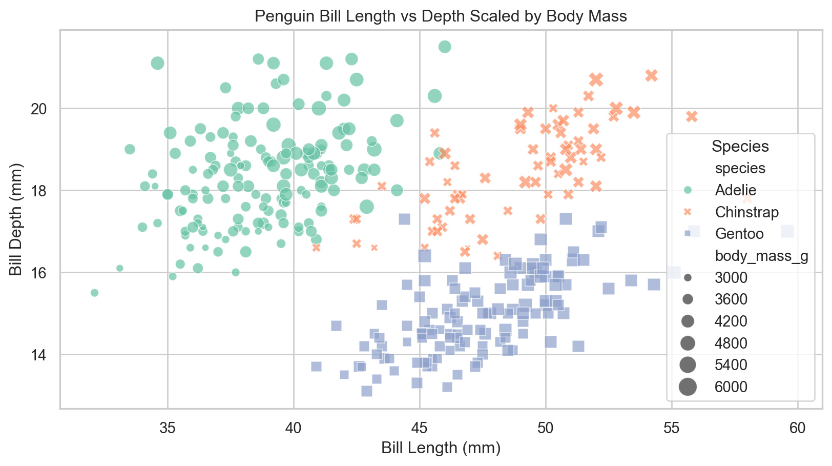
We can also format using continuous variables!

For our scatter plot suppose we wish to also incorporate the influence of body mass on bill length and depth.
We can use the size and sizes parameters to control the size of points based on body mass.

How about this scatter plot?

ax = sns.scatterplot(
    x="bill_length_mm", y="bill_depth_mm",
    data=penguins,
    hue="species",                           # Color by species 
    style="species",                         # Shape by species
    size="body_mass_g",                      # Scale by body mass
    sizes=(20, 200),                         # Set size range
    alpha=0.7                                # Set point transparency
)
ax.set(xlabel="Bill Length (mm)", ylabel="Bill Depth (mm)", title="Penguin Bill Length vs Depth Scaled by Body Mass")
ax.legend(title="Species")
plt.show()

Continuous Variable Formatting

Scatter plot of bill length vs bill depth scaled by body mass for the penguins dataset. (`seaborn`)

Multiplotting

What is multiplotting?

Particularly for reports we often are interested in showing multiple related visualizations together.
In matplotlib we can use the subplots() function to create multiple plots in a single figure.
In seaborn we can use the FacetGrid() function to create a grid of plots based on the values of one or more categorical variables.
- This is where the improved efficiency of seaborn becomes apparent as we can create complex multiplots with very little code.

Multiplots with `matplotlib`

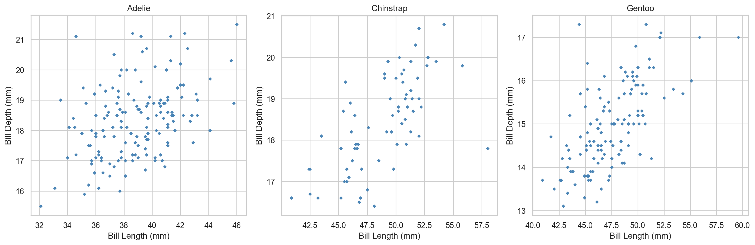
It’s still important to learn the syntax

We first create a figure with multiple axes using plt.subplots().
We then loop through the axes and create a scatter plot for each species in the penguins dataset.
Finally, we adjust the layout and display the plot.

Starting to get confusing! 😵‍💫

fig, axes = plt.subplots(nrows=1, ncols=3, figsize=(15, 5))     # Create figure and axes objects
species = penguins["species"].unique()              # Get unique species

for ax, sp in zip(axes, species):                            # Loop through axes and species
    subset = penguins[penguins["species"] == sp]             # Subset data for each species
    ax.scatter(                                              # Create scatter plot
        subset["bill_length_mm"], subset["bill_depth_mm"],
        color="steelblue",                          
        alpha=0.95,                                 
        s=7,                                        
        marker="D"                                  
    )
    ax.set_title(sp)                             
    ax.set_xlabel("Bill Length (mm)")            
    ax.set_ylabel("Bill Depth (mm)")             
plt.tight_layout()                          # Adjust layout
plt.show()

Multiplots with `matplotlib`

Multiplot of bill length vs bill depth for each species in the penguins dataset. (`matplotlib`)

Multiplots with `seaborn`

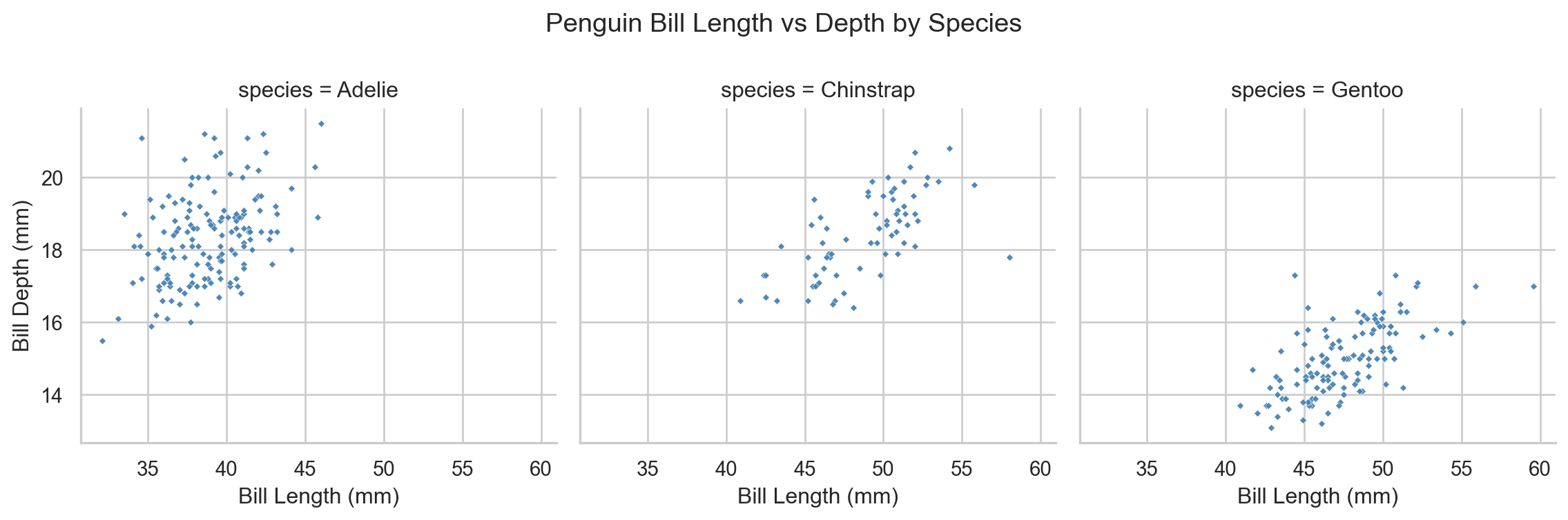
So much easier! 😎

We can create the same multiplot using seaborn’s FacetGrid() function with much less code.
This function allows us to create a grid of plots based on the values of one or more categorical variables, making it easy to compare relationships across different groups.
The map() method is used to apply a plotting function (e.g., sns.scatterplot) to each subset of the data defined by the grid.

Facets with `seaborn`

g = sns.FacetGrid(
  penguins, 
  col="species", 
  height=4, 
  aspect=1)  # Create facet grid
g.map(
  sns.scatterplot, 
  "bill_length_mm", "bill_depth_mm", 
  color="steelblue", 
  alpha=0.95, 
  s=7, 
  marker="D")  # Map scatter plot to each facet
g.set_axis_labels(
  "Bill Length (mm)", 
  "Bill Depth (mm)"
  )  # Set axis labels
g.fig.subplots_adjust(top=0.8)  # Adjust subplot spacing
g.fig.suptitle("Penguin Bill Length vs Depth by Species")  # Set overall title
plt.show()  # Show the plot

Multiplots with `seaborn`

Multiplot of bill length vs bill depth for each species in the penguins dataset. (`seaborn`)

Conclusion

✅ What we covered

Standard visualizations and when to use them.
Basic visualization production in matplotlib and seaborn.
Style and formatting features including themes, variable formatting, and facets.
The importance of creativity and experimentation in data visualization.
Facets.

📅 What’s next?

Exploratory Data Analysis (EDA).
Descriptive statistics.
Complex seaborn visualizations.
Interactive visualizations with altair.

Lecture 5: Data Visualization

🚁 Overview

Aims of the lecture

📚 Required Libraries

Recap: Data Preparation

Data Preparation

Next Step: Exploration

Exploratory Data Analysis (EDA)

🔍 Exploratory Data Analysis (EDA)

What is EDA?

EDA Steps (Topic of next lecture)

Data Visualization

Data Visualization

Data Visualization

Why Visualize Data?

Principles of Effective Data Visualization

Types of Visualization

Exploratory vs Presentation

Static vs Interactive vs Animated

Visualizations in Python

matplotlib

seaborn

altair

Plan for upcoming lectures

Lecture 5 (Today)

Lecture 6 (Thursday)

Basic Visualizations

Standard Visualizations

Example Data: penguins

Object-Oriented Interface

Pyplot vs Object-Oriented Interface

Only covering the basics of matplotlib

matplotlib Scatter Plots

Scatter Plots

matplotlib Scatter Plots

seaborn Scatter Plots

What makes seaborn so great?

Scatter Plots in seaborn

seaborn Scatter Plots

Variable Based Formatting

Variable Based Formatting

Scatter Plots with Variable Based Formatting in seaborn

Variable Based Formatting

Adding Best Fit Lines

What are best fit lines?

seaborn Regression Lines

Adding Best Fit Lines

Bar Plots

What are bar plots?

matplotlib Bar Plots

Bar Plots

Count Plots

seaborn Count Plots

Count Plots

Subgrouping and Variable Formatting

Subgrouping

Subgrouped Bar Plot with Variable Formatting

Subgrouping and Variable Formatting

Box Plots

What are box plots?

seaborn Box Plots

Box Plots

Histograms

What are histograms?

seaborn Histograms

Histograms

Histograms with Variable Formatting and Kernel Density Estimates

Let’s start exploring what we can do!

seaborn Histograms with KDEs

Histograms with Variable Formatting and Kernel Density Estimates

Violin Plots

Fancy box plots?

Violin Plots in seaborn

Violin Plots

Advanced Visualizations

Advanced Visualizations

Be creative!

Perhaps this boxplot is more informative?

Advanced Visualizations

Continuous Variable Formatting

`matplotlib`

`seaborn`

`altair`

Example Data: `penguins`

Only covering the basics of `matplotlib`

`matplotlib` Scatter Plots

`matplotlib` Scatter Plots

`seaborn` Scatter Plots

What makes `seaborn` so great?

Scatter Plots in `seaborn`

`seaborn` Scatter Plots

Scatter Plots with Variable Based Formatting in `seaborn`

`seaborn` Regression Lines

`matplotlib` Bar Plots

`seaborn` Count Plots

`seaborn` Box Plots

`seaborn` Histograms

`seaborn` Histograms with KDEs

Violin Plots in `seaborn`

Multiplots with `matplotlib`

Multiplots with `matplotlib`

Multiplots with `seaborn`

Facets with `seaborn`

Multiplots with `seaborn`