Lecture 2: Data Structure

PSTAT100: Data Science - Concepts and Analysis

John Inston

johninston@ucsb.edu

University of California, Santa Barbara

April 7, 2026

🚁 Overview

Aims of the lecture

Introduce data handling in Python.
- numpy arrays.
- pandas DataFrames.
Data Structures.
- Wide vs Long.
- Converting between long and wide data structures.
- pd.melt and pd.pivot.
Tidy Data.
- Tidy Data Principles.

Data in Python

🐍 Python Basics

Python Variables

Python is a general purpose programming language.
Python natively stores data in variables of different types:
- Strings (str) - text data.
- Integers (int) - whole numbers.
- Floating point numbers (float) - decimal numbers.
- Booleans (bool) - true/false values.
- Lists (list) - ordered collections of data.
- Dictionaries (dict) - key-value pairs.
- Tuples (tuple) - ordered, immutable collections of data.
- Sets (set) - unordered collections of unique data.
Packages such as pandas and numpy provide additional data types and functions for working with data such as:
- Pandas DataFrames (.DataFrame) - tabular data.
- Numpy arrays (.array) - numerical data.

Python Syntax

Built-in Data Types

my_string = "Hello, World!"
my_integer = 10
my_float = 3.14
my_boolean = True
my_list = [1, 2, 3, 4, 5]
my_tuple = (1, 2, 3, 4, 5)
my_set = {1, 2, 3, 4, 5}
my_dict = {"name": "John", "age": 30}

item_list = [my_string, my_integer, my_float, my_boolean,
             my_list, my_tuple, my_set, my_dict]

for item in item_list:
    print(type(item), ":", item)

<class 'str'> : Hello, World!
<class 'int'> : 10
<class 'float'> : 3.14
<class 'bool'> : True
<class 'list'> : [1, 2, 3, 4, 5]
<class 'tuple'> : (1, 2, 3, 4, 5)
<class 'set'> : {1, 2, 3, 4, 5}
<class 'dict'> : {'name': 'John', 'age': 30}

Built-in data types have limitations:
- Scalability (inefficient memory usage).
- Functionality (e.g. vector operations, manipulation).

my_list + 2

---------------------------------------------------------------------------
TypeError                                 Traceback (most recent call last)
Cell In[2], line 1
----> 1 my_list + 2

TypeError: can only concatenate list (not "int") to list

NumPy

NumPy Arrays

Numpy arrays are \(n\)-dimensional arrays of homogeneous data.
- Vectorized operations.
- Efficient memory usage.
Make sure you are familiar with the basics of NumPy arrays:
- Construction: array, linspace, full, etc.
- Indexing / Slicing.
- Broadcasting.

import numpy as np

list_array = np.array([1, 2, 3, 4, 5])
linspace_array = np.linspace(0, 1, 5)

print(list_array)
print(linspace_array)

list_array[:3]
linspace_array[list_array > 2]

[1 2 3 4 5]
[0.   0.25 0.5  0.75 1.  ]

array([0.5 , 0.75, 1.  ])

Pandas DataFrames

🐼 What is Pandas?

Pandas is a library for data manipulation and analysis.
- Provides data structures and functions for working with tabular data.
- Built on top of NumPy.

Pandas DataFrames

Pandas DataFrames are 2-dimensional tabular data structures with labeled rows and columns.
- They are similar to NumPy arrays but with labeled axes.
- They are similar to dictionaries but with labeled columns.

import pandas as pd

# Constructing a dataframe
data = pd.DataFrame({
    "name": ["John", "Jane", "Jim", "Jill"],
    "age": [20, 21, 22, 23],
    "city": ["New York", "Los Angeles", 
        "Chicago", "Houston"]
})

print(data)

   name  age         city
0  John   20     New York
1  Jane   21  Los Angeles
2   Jim   22      Chicago
3  Jill   23      Houston

📂 Loading Data Files

Data Formats

In this course we will primarily use tabular data stored in the following file formats:
- Text files (.txt) - simplest format but with loading challenges
- Comma Separated Values files (.csv) - most common format.
- Tab Separated Values files (.tsv) - similar to CSV but uses tabs instead of commas.
- Excel files (.xlsx) - spreadsheets with complex formulas and formatting.

Loading `.csv` files and `.xlsx` files

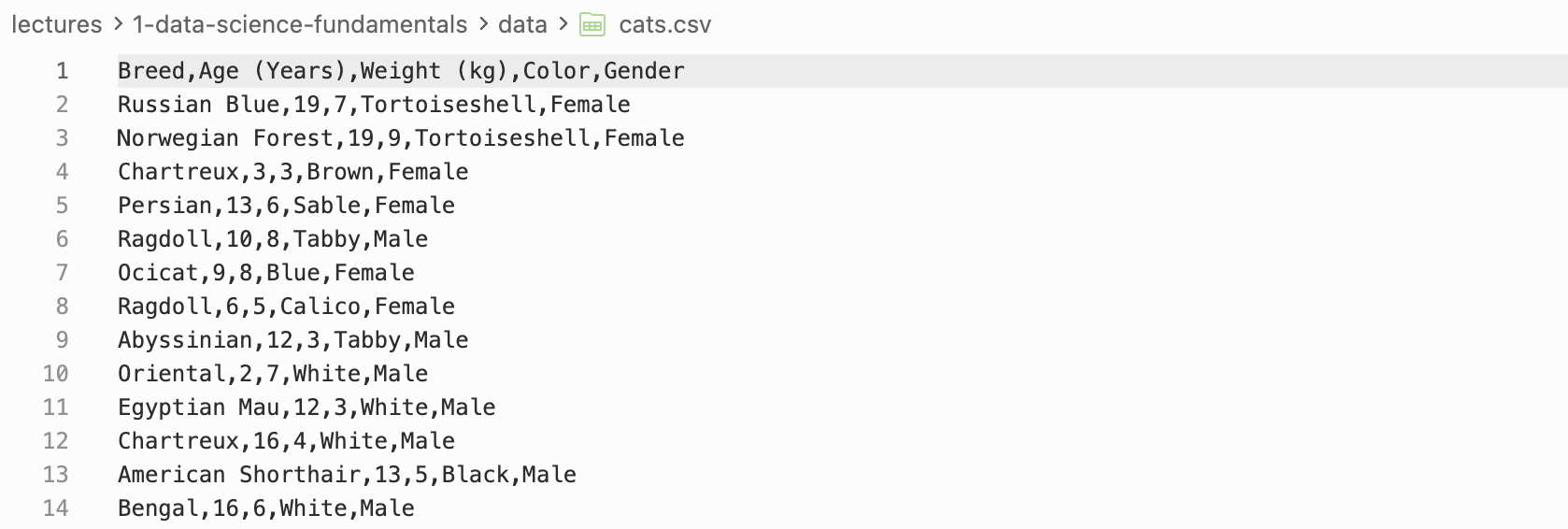
`.csv` files

.csv files are comma separated values files and are commonly used to store tabular data.
To load a .csv file we can use the pd.read_csv function.

cats_data = pd.read_csv("data/cats.csv")
print(cats_data.head())

              Breed  Age (Years)  Weight (kg)          Color  Gender
0      Russian Blue           19            7  Tortoiseshell  Female
1  Norwegian Forest           19            9  Tortoiseshell  Female
2         Chartreux            3            3          Brown  Female
3           Persian           13            6          Sable  Female
4           Ragdoll           10            8          Tabby    Male

`.xlsx` files

.xlsx files are Excel files and are commonly used to store tabular data.
To load a .xlsx file we can use the pd.read_excel function.

sales_data = pd.read_excel(
    "data/office_sales.xlsx", 
    sheet_name="SalesOrders")
print(sales_data.head())

   OrderDate   Region      Rep    Item  Units  Unit Cost   Total
0 2024-01-06     East    Jones  Pencil     95       1.99  189.05
1 2024-01-23  Central   Kivell  Binder     50      19.99  999.50
2 2024-02-09  Central  Jardine  Pencil     36       4.99  179.64
3 2024-02-26  Central     Gill     Pen     27      19.99  539.73
4 2024-03-15     West  Sorvino  Pencil     56       2.99  167.44

⋙ Dataframe Basics

Manipulation and Indexing

There are many ways we can manipulate dataframes including:
- Finding dataframe information with functions like columns, index, shape, head, tail, etc.
- Indexing / Slicing / Filtering. (.loc, .iloc)
- Adding / Removing columns and rows. (.drop, .dropna, .insert, .concat)
- Sorting. (.sort_values, .sort_index)

# Properties
print(cats_data.columns)
print(cats_data.index)
print(cats_data.shape)

Index(['Breed', 'Age (Years)', 'Weight (kg)', 'Color', 'Gender'], dtype='object')
RangeIndex(start=0, stop=1000, step=1)
(1000, 5)

# Indexing 
print(cats_data[["Breed", "Color"]].head())
print(cats_data.iloc[3:5])

              Breed          Color
0      Russian Blue  Tortoiseshell
1  Norwegian Forest  Tortoiseshell
2         Chartreux          Brown
3           Persian          Sable
4           Ragdoll          Tabby
     Breed  Age (Years)  Weight (kg)  Color  Gender
3  Persian           13            6  Sable  Female
4  Ragdoll           10            8  Tabby    Male

# Adding / Removing columns and rows
cats_data_dropped = cats_data.drop(columns=["Color"])
print(cats_data_dropped.columns)

Index(['Breed', 'Age (Years)', 'Weight (kg)', 'Gender'], dtype='object')

🏢 Data Structure

🏗️ Different Data Structures

Often two data sets can have the same semantics but different data structures.
Data structures can be broadly categorized into two types:

Wide data structure:
- One row per subject.
- Repeated measurements are in separate columns.

Long data structure:
- One row per measurement.
- There is a column identifying which variable was measured

↔︎️ Wide Data Structure

Let’s build some intuition…

To build our intuition let’s create a copy of the data set used by Luke Bennett.
- The data set contains the points, assists and rebounds of 4 basketball teams.
- ❓ Have a go at making this dataframe in python using pd.DataFrame.

Basketball Data Set
	points	assists	rebounds
team
A	88	12	22
B	91	17	28
C	99	24	30
D	94	28	31

Each observation (team) is on its own row.
Each observation has multiple variables in separate columns.

↕️ Long Data Structure

What is a long data structure?

What would this data look like in a long data structure?

	statistic	value
team
A	points	88
A	assists	12
A	rebounds	22
B	points	91
B	assists	17
B	rebounds	28

We observe now that:
- Each measurement has its own row (value)
- There is a column identifying which variable was measured (statistic)

Long vs Wide Data Structure

🤔 Which is better?

Wide data is more human-readable:
- Common in spreadsheets
Long data is more computer-readable:
- Required by most plotting libraries (seaborn, ggplot in R)
- Easier to filter, group, and aggregate in pandas.
It is therefore important to be able to convert between the two data structures.

Code to build the basketball data set

basketball_data = pd.DataFrame({
    "team": ["A", "B", "C", "D"],
    "points": [88, 91, 99, 94],
    "assists": [12, 17, 24, 28],
    "rebounds": [22, 28, 30, 31]
})

`pd.melt`

`pd.melt` - Wide → Long

pd.melt is a function that converts a wide data structure to a long data structure.
It takes the following arguments:
- id_vars are the columns that identify the subject.
- var_name is the name of the column that will contain the variable names.
- value_name is the name of the column that will contain the variable values.

# Wide → Long
basketball_data_long = basketball_data.melt(
    id_vars=["team"], 
    var_name="statistic", 
    value_name="value"
    )
print(basketball_data_long)

   team statistic  value
0     A    points     88
1     B    points     91
2     C    points     99
3     D    points     94
4     A   assists     12
5     B   assists     17
6     C   assists     24
7     D   assists     28
8     A  rebounds     22
9     B  rebounds     28
10    C  rebounds     30
11    D  rebounds     31

`pd.pivot`

`pd.pivot` - Long → Wide

pd.pivot is a function that converts a long data structure to a wide data structure.
It takes the following arguments:
- index is the column that will contain the subject identifiers.
- columns is the column that will contain the variable names.
- values is the column that will contain the variable values.

# Long → Wide
basketball_data_wide = basketball_data_long.pivot(
    index="team", 
    columns="statistic", 
    values="value")
print(basketball_data_wide)

statistic  assists  points  rebounds
team                                
A               12      88        22
B               17      91        28
C               24      99        30
D               28      94        31

Lack of Standard Format

Which do you prefer?

Difficult to say why one layout might be preferable.
- Most data is stored in a layout that made intuitive sense to the creator.
- 🙂‍↔︎️ Idiosyncratic and unprincipled.
- Few widely used conventions
- Lots of variability ‘in the wild’

Consequences for Data Scientists

Data scientists must determine how best to reorganize datasets.
Broadly, this involves two interdependent choices:

Choice of representation: how to encode information.
- Dates as one or three variables?
- Use values 1, 2, 3 or ‘low’, ‘med’, ‘high’?

Choice of form: how to display information
- Wide table or long table?
- One table or many?

What’s the solution?

🧹Tidy Data Standard

Data scientists introduced the tidy data standard to help solve the problem of inconsistent data structures.
It has two main advantages:
- Facilitates workflow by establishing a consistent dataset structure.
- Principles are designed to make transformation, exploration, visualization, and modeling easy.

Tidy Data

Tidy Data Principles

What is tidy data?

“Tidying your data means storing it in a consistent form that matches the semantics of the dataset with the way it is stored. In brief, when your data is tidy, each column is a variable, and each row is an observation. Tidy data is important because the consistent structure lets you focus your struggle on questions about the data, not fighting to get the data into the right form for different functions.” - Wickham and Grolemund, R for Data Science, 2017.

Tidy = Semantics and Structure

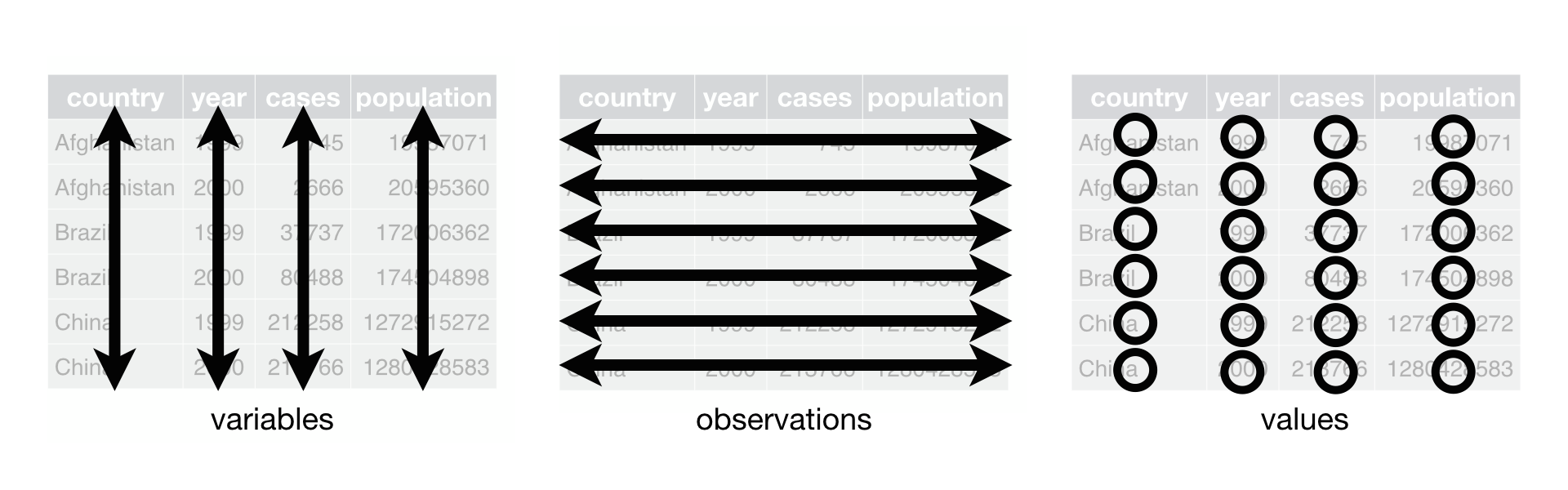
A dataset is a collection of values which is said to have:
- Semantics: Meaning of each value
- Structure: How values are arranged
The tidy standard: data semantics \(\leftrightarrow\) data structure

🧹 Tidy Data Standard

Tidy Data Definition

Tidy Data Standard

For data to be tidy, it must satisfy the following three rules:

Each variable is a column.
Each observation is a row.
Each type of observational unit forms a table.

Tidy or Not - Example 1

Is this tidy?

For our first example let’s look at World Bank data on annual GDP growth.
- We load this data from a .csv file using pd.read_csv.
- We look at the dimensions of the dataframe using shape.

gdp = pd.read_csv('data/annual_growth.csv', encoding = 'latin1')
print(gdp.shape)
gdp.head()

(264, 61)

Tidy or Not? Example 1
	Country Name	Country Code	1961	1962	1963	1964	1965	1966	1967	1968	...	2010	2011	2012	2013	2014	2015	2016	2017	2018	2019
0	Aruba	ABW	NaN	NaN	NaN	NaN	NaN	NaN	NaN	NaN	...	-3.685029	3.446055	-1.369863	4.198232	0.300000	5.700001	2.100000	1.999999	NaN	NaN
1	Afghanistan	AFG	NaN	NaN	NaN	NaN	NaN	NaN	NaN	NaN	...	14.362441	0.426355	12.752287	5.600745	2.724543	1.451315	2.260314	2.647003	1.189228	3.911603
2	Angola	AGO	NaN	NaN	NaN	NaN	NaN	NaN	NaN	NaN	...	4.403933	3.471976	8.542188	4.954545	4.822628	0.943572	-2.580050	-0.147213	-2.003630	-0.624644
3	Albania	ALB	NaN	NaN	NaN	NaN	NaN	NaN	NaN	NaN	...	3.706892	2.545322	1.417526	1.001987	1.774487	2.218752	3.314805	3.802197	4.071301	2.240070
4	Andorra	AND	NaN	NaN	NaN	NaN	NaN	NaN	NaN	NaN	...	-1.974958	-0.008070	-4.974444	-3.547597	2.504466	1.434140	3.709678	0.346072	1.588765	1.849238

5 rows × 61 columns

Compare Semantics and Structure

Tidy or Not? Example 1
	Country Name	Country Code	1961	1962	1963	1964	1965	1966	1967	1968	...	2010	2011	2012	2013	2014	2015	2016	2017	2018	2019
0	Aruba	ABW	NaN	NaN	NaN	NaN	NaN	NaN	NaN	NaN	...	-3.685029	3.446055	-1.369863	4.198232	0.300000	5.700001	2.100000	1.999999	NaN	NaN
1	Afghanistan	AFG	NaN	NaN	NaN	NaN	NaN	NaN	NaN	NaN	...	14.362441	0.426355	12.752287	5.600745	2.724543	1.451315	2.260314	2.647003	1.189228	3.911603
2	Angola	AGO	NaN	NaN	NaN	NaN	NaN	NaN	NaN	NaN	...	4.403933	3.471976	8.542188	4.954545	4.822628	0.943572	-2.580050	-0.147213	-2.003630	-0.624644
3	Albania	ALB	NaN	NaN	NaN	NaN	NaN	NaN	NaN	NaN	...	3.706892	2.545322	1.417526	1.001987	1.774487	2.218752	3.314805	3.802197	4.071301	2.240070
4	Andorra	AND	NaN	NaN	NaN	NaN	NaN	NaN	NaN	NaN	...	-1.974958	-0.008070	-4.974444	-3.547597	2.504466	1.434140	3.709678	0.346072	1.588765	1.849238

5 rows × 61 columns

Semantics		Structure
Observations: Variables: Observational units:	Annual records GDP growth and year Countries	Rows: Columns: Tables:	Countries Value of year Just one

❌ Rules 1 and 2 are violated since column names are values, not variables.
- Conclusion: No, this is not tidy. 👎

Tidy or Not - Example 1

Let’s see if we can make it tidy…

The things we wish to change are:
- Set the index column to be country name using set_index.
- Drop the country code column (personal preference but superfluous) using drop.
- Melt the data so that year and growth rate are variables (columns), with one row per country per year, using melt.
- Sort the data by year and country name using sort_values.

gdp_tidy = gdp.set_index(
    'Country Name'
).drop(
    columns = 'Country Code'
).melt(
    var_name = 'year',
    value_name = 'growth_pct',
    ignore_index = False
).reset_index(
).sort_values(
    ['year', 'Country Name']
).set_index('Country Name')

Were we successful?

Tidy or Not? Example 1
	year	growth_pct
Country Name
Afghanistan	1961	NaN
Albania	1961	NaN
Algeria	1961	-13.605441
American Samoa	1961	NaN
Andorra	1961	NaN

Semantics		Structure
Observations: Variables: Observational units:	Annual records GDP growth and year Countries	Rows: Columns: Tables:	Annual records GDP growth and year Just one

✅ All three rules are satisfied. Rows are observations, columns are variables, and there is one unit type and one table.
- Conclusion: Yes, we were successful! 🎉

Conclusion

✅ What we covered

Python data types, NumPy, and pandas.
numpy and pandas
Data Structure
Wide vs Long
Tidy Data

📅 What’s next?

Detailed data preparation!

Lecture 2: Data Structure

🚁 Overview

Aims of the lecture

Data in Python

🐍 Python Basics

Python Variables

Python Syntax

Built-in Data Types

NumPy

NumPy Arrays

Pandas DataFrames

🐼 What is Pandas?

Pandas DataFrames

📂 Loading Data Files

Data Formats

Loading .csv files and .xlsx files

.csv files

.xlsx files

⋙ Dataframe Basics

Manipulation and Indexing

🏢 Data Structure

🏗️ Different Data Structures

↔︎️ Wide Data Structure

Let’s build some intuition…

↕️ Long Data Structure

What is a long data structure?

Long vs Wide Data Structure

🤔 Which is better?

Code to build the basketball data set

pd.melt

pd.melt - Wide → Long

pd.pivot

pd.pivot - Long → Wide

Lack of Standard Format

Which do you prefer?

Consequences for Data Scientists

What’s the solution?

🧹Tidy Data Standard

Tidy Data

Tidy Data Principles

What is tidy data?

Tidy = Semantics and Structure

🧹 Tidy Data Standard

Tidy Data Definition

Tidy or Not - Example 1

Is this tidy?

Compare Semantics and Structure

Tidy or Not - Example 1

Let’s see if we can make it tidy…

Were we successful?

Conclusion

✅ What we covered

📅 What’s next?

References

Loading `.csv` files and `.xlsx` files

`.csv` files

`.xlsx` files

`pd.melt`

`pd.melt` - Wide → Long

`pd.pivot`

`pd.pivot` - Long → Wide