Lecture 1: Data Science Fundamentals

PSTAT100 Data Science Concepts and Analysis

John Inston

University of California, Santa Barbara

April 7, 2026

Course Introduction

πŸ‘‹ Introduction

Welcome to PSTAT100 Data Science Concepts and Analysis! πŸŽ‰

🀝 About Me

  • My name is John Inston.
    • Pronouns: I use he/him/his pronouns.
  • I am a 4th year PhD candidate πŸ‘΄ in the Department of Statistics and Applied Probability.
  • My research interests include stochastic games 🎲 and numerical optimization πŸ’».


πŸ“§ Contact Information

βœ‰οΈ Email: johninston@ucsb.edu

🌐 Website: johnrobininston.com

Office Hours

🏒 OH: South Hall 5431T R 1PM to 3PM.

πŸ‘©β€πŸ« Teaching Staff

I am being assisted this term by the following wonderful teaching assistants:

  • Lauren Hughes

  • Yuting Ma

  • Zhuojun Lyu

    • Pronouns: she/her/hers
    • βœ‰οΈ Email: zhuojun@ucsb.edu
    • 🏒 OH: TBD.

❗ Due to space availability section switching must be confirmed in advance with your TA.

ℹ️ Prerequisites

Programming Language

  • This course will be taught in python 🐍.
    • A working knowledge of python is not required but it is expected that you have some familiarity with similar programming languages.
    • You are also expected to create documents using Jupyter notebooks or Quarto markdown.

Prerequisite Courses

  • PSTAT 120A
    • Probability Theory
    • Statistics
  • CS 9 or CS 16
    • Python Programming
    • Data Structures
    • Algorithms
  • Math 4A
    • Linear Algebra

πŸ“ Supplementary materials summarizing these topics will be made available in the online lecture notes for review.

ℹ️ Course Information

πŸ“ Course Materials

  • You will be provided with:
    • πŸ“ Lecture Notes (slides, online, pdf)
    • πŸ“š Suggested reading (textbooks, online notebooks)
    • πŸ§ͺ Lab and assignment solutions
  • You can access all course material through the Canvas page.
    • All material that is not assessed will also be made available on the course website.

πŸ‘©β€βš–οΈ Course Policies

  • Communication is key! πŸ’¬

  • No plagiarism! ❌

  • πŸ€– AI tools are encouraged for learning.

  • Be respectful. 🀝

Please make sure to read through the course policies detailed in the syllabus.

πŸ“ Assessments

πŸ“ Assignments (40%)

  • 4 assignments throughout the quarter.
    • These will be released and submitted on Canvas
    • Due at the end of weeks 2, 4, 6, and 8.

πŸ’» Labs (30%)

  • 8 lab worksheets
    • Submitted to Canvas by the end of the week.
    • In lab sessions your TA will help you with problems.

πŸ“Š Project (30%)

  • You are required to complete a data analysis project.
    • Individual or group.
    • Details of this project will be specified in the coming weeks.

βœ… Topic Outline

The following is a tentative course outline:

  1. Introduction to Data Science
    • Python Fundamentals
    • Data Lifecycle
  2. Data Preparation
    • Data Cleaning
    • Missingness
  3. Exploratory Data Analysis
    • Data Visualization
    • Data Summarization
  4. Statistical Foundations
    • Probability
    • Hypothesis Testing
  1. Regression
    • Simple / Multiple Linear Regression
    • Ridge / Lasso / Elastic Net Regression
  2. Classification Methods
    • Logistic Regression
    • Support Vector Machines
  3. Tree-Based Methods
    • Decision Trees / Random Forests
  4. Unsupervised Learning
    • PCA & Clustering
  5. Introduction to Deep Learning
  6. Data Science Ethics
    • Privacy, Fairness and Bias

πŸ“ˆ Maximizing Your Learning

πŸ’Ό Professional Skills

In addition to technical topics we will also develop your professional skills as a data scientist including:

  • Technical document production.
  • πŸ—£οΈ Precise and clear communication.
  • 🀝 Collaboration and team work.
  • Version control (GitHub).
  • Independent learning.

🎯 Course Aims

Your course aims should be:

  • πŸ› οΈ Build a toolkit for your future career.
  • Independently learning new tools and techniques based on the problem at hand.
  • To have a project to showcase your skills and knowledge for job applications.
    • And have the start of a project portfolio on GitHub!

πŸ’ͺ Python Bootcamp

What about if I am not familiar with Python? πŸ€”


When and Where?

I will be hosting a Python Bootcamp this Thursday from 1:00pm to 3:00pm in South Hall 5421.

❗ Attendance is optional!

Who is this for?

  • Encouraged for anybody who is unfamiliar with Python or needs a refresher.
  • Focus will be on IDE setup, basic functionality and document creation.

Data Science Fundamentals

πŸ“Š Data Science

What is Data Science?

Let’s see what Claude thinks:

Claude’s Definition of Data Science.

Fundamental Aims

Simply put…

Data science is the practice of using data to extract insights and knowledge. πŸ‘

How does it work?

  • Data science is an interdisciplinary field, requiring:
    • Statistics
    • Mathematics
    • Computer science
    • Domain knowledge
  • Required to manage and interpret large, complicated data sets.

πŸ€” Notice that these disciplines loosely correspond to the prerequisites for this course.

Data Science Disciplines

Intersection of the Disciplines

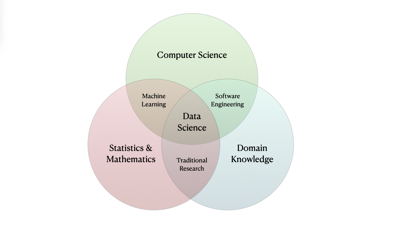
Data Science Venn Diagram.

πŸ”’ Data

What is Data?

Definition: Data

Data is (digital) information (such as measurements or statistics) used as a basis for reasoning, discussion, or calculation.

  • Raw data is often difficult or even impossible to interpret.
    • Hence, the need for Data Science!

For example…

Data Growth

🫩 Sooo much data!

  • The amount of data being collected, stored, and processed is growing exponentially!

  • Larger variety of increasingly complicated data types.

Worldwide Data Growth.

πŸ”’ Datasets

Datasets

Definition: Dataset

A dataset is a collection of observations taken on observational units, consisting of values measured on a set of variables.

Terminology

  • An observational unit is the entity that is being measured.
    • People in a study, cars on a production line, etc.
  • An observation is a collection of values (e.g. a vector) measured on various variables.
    • One person, car in particular is an observation.
    • Variables might be the person’s age, the car’s engine size, etc.

Let’s look at our first example dataset.

Dataset Example - cats.csv

🐈 A New Cat Dataset

First 5 rows of cats.csv
Breed Age (Years) Weight (kg) Color Gender
0 Russian Blue 19 7 Tortoiseshell Female
1 Norwegian Forest 19 9 Tortoiseshell Female
2 Chartreux 3 3 Brown Female
3 Persian 13 6 Sable Female
4 Ragdoll 10 8 Tabby Male


Identifying Observations and Variables

  • The cats dataset was provided by Waqar Ali on Kaggle.

  • Here the observational unit is a cat.

  • This dataset of 1000 observations (rows, individual cats) each with 5 variables (columns).

Semantics vs Structure

What is the difference?

  • In general, we distinguish between the semantics and structure of a dataset.

  • The semantics of a dataset refers to the meaning behind the data.

    • Interpretation and representation.
  • The structure of a dataset refers to the way the data is organized.

    • Shape, organization and storage.
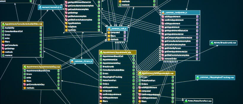
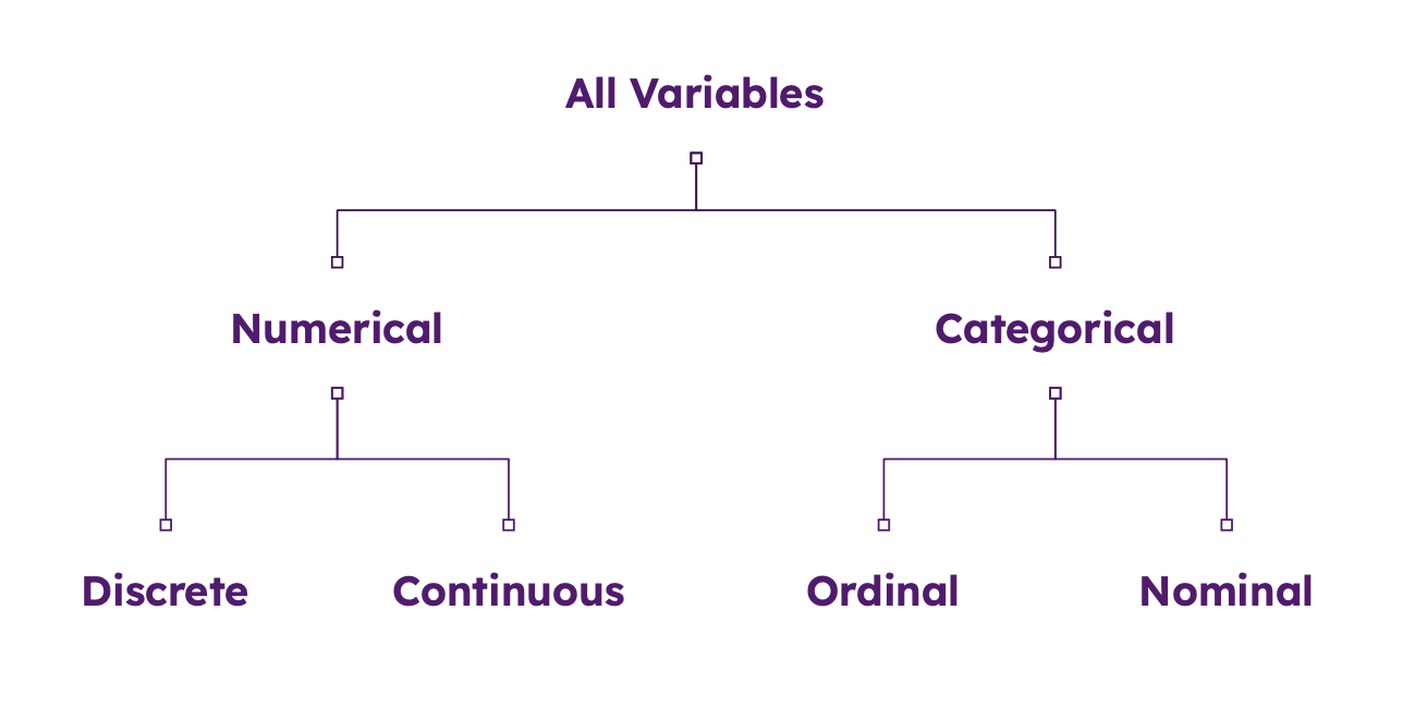
πŸ”’ Types of Data

πŸ”’ Quantitative Data

  • Quantitative Data (Numerical): Represents measurable quantities.
    • Discrete: Counted items that are distinct and whole (e.g., number of children, product sales).
    • Continuous: Measured items that can be any value within a range (e.g., height, weight).

βš–οΈ Qualitative Data

  • Qualitative Data (Categorical): Represents descriptive characteristics or labels.
    • Nominal: Named categories with no inherent order (e.g., gender, hair color, blood type).
    • Ordinal: Categories with a logical order or ranking (e.g., satisfaction surveys, education level).

🏒 Structured vs. Unstructured Data

  • Structured vs. Unstructured Data:
    • Structured: Organized, formatted data (e.g., Excel sheets, SQL databases).
    • Unstructured data: Data without a fixed schema (e.g., video, audio, free text).

Data Type Example - cats.csv

🐈 The Cats Strike Back!

First 5 rows of cats.csv
Breed Age (Years) Weight (kg) Color Gender
0 Russian Blue 19 7 Tortoiseshell Female
1 Norwegian Forest 19 9 Tortoiseshell Female
2 Chartreux 3 3 Brown Female
3 Persian 13 6 Sable Female
4 Ragdoll 10 8 Tabby Male

Identifying Variable Types

  • The Breed, Color, and Gender variables are qualitative variables since they are categorical.

  • The Age and Weight variables are quantitative variables since they are numerical.

    • Both are continuous variables since they can take on any value within a range.
    • ❗ We note however that they have both been discretized into bins.

πŸ”„ Transformations

Variable Transformations

  • Variables can be transformed from one type to another, often for:
    • Improved interpretability.
    • Removing excessive detail.
    • Subsequent analysis (e.g. PCA).

🐈 Return of the Cat Dataset

Suppose we are interested in transforming the quantitative age variable into the categories young, middle-aged, and senior.

  • We create a new variable AgeGroup with the following values:
    • Young: 0-5 years
    • Middle-Aged: 6-10 years
    • Senior: 11+ years

Transformations Example - cats.csv

πŸ• Transformed Cat Dataset

First 5 rows of cats.csv with AgeGroup variable
Breed Age (Years) Weight (kg) Color Gender AgeGroup
0 Russian Blue 19 7 Tortoiseshell Female Senior
1 Norwegian Forest 19 9 Tortoiseshell Female Senior
2 Chartreux 3 3 Brown Female Young
3 Persian 13 6 Sable Female Senior
4 Ragdoll 10 8 Tabby Male Middle-Aged

Interpretation of the Transformed Variable

  • We have now transformed the numerical Age (Years) variable into a qualitative AgeGroup variable.

  • We will revisit variable transformations in more detail later in the course when we discuss data preparation.

Data Type Hierarchy

Variable Classification.

πŸ”’ Tabular Data

  • We will primarily be working with tabular data.
    • Spreadsheet style datasets containing both quantitative and qualitative data.
    • We will occasionally deal with more complex structures such as databases.

Complicated Data

πŸ˜΅β€πŸ’« More Complicated Data Types

In reality there is a wide variety of different data types:

  • Time series data - stock prices, weather patterns, etc.
  • Spatial data - map data, satellite imagery, etc.
  • Textual data - social media posts, news articles, etc.
  • Image data - photos, videos, etc.
  • Audio data - audio recordings, podcasts, etc.
  • Video data - videos, etc.
  • Network / graphical data - social media networks, etc.


Each data type has its own unique set of challenges and techniques for data scientists to apply.

Complicated Data Example - MNIST

πŸ–οΈ Handwritten Digits

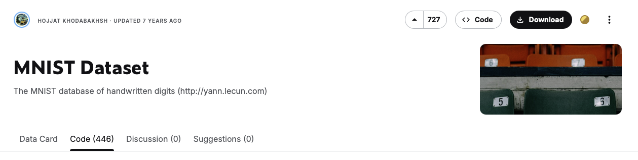
MNIST database, a subset of the larger NIST made available by Yann LeCun on Kaggle.

  • The database is of handwritten digits.
    • White text on a black background.
  • The data is complicated!
    • There are 70,000 observations total (60,000 training and 10,000 testing).
    • Each observation consists of 28x28 pixels, with a total of 784 pixels per observation.
    • Each pixel is a grayscale value between 0 and 255 (0 = black, 255 = white).

Handwritten Digits

πŸ–οΈ Handwritten Digits

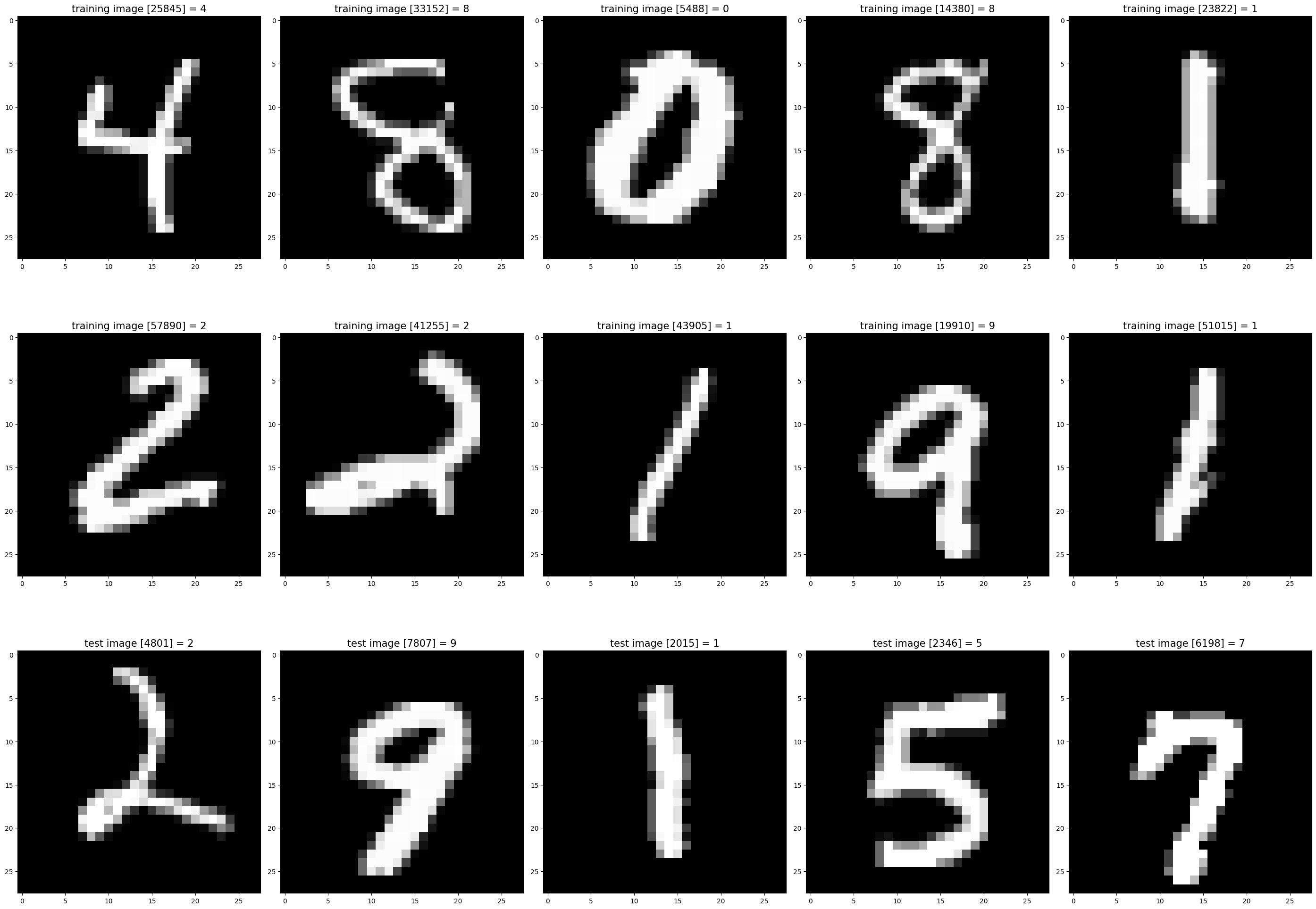
MNIST Data Visualization.

πŸ“– Data Literacy

My point is…

The world of data is confusing! πŸ˜΅β€πŸ’«

  • Different data types with different formats and different dimensions.
  • Each has unique challenges and techniques for data scientists to learn.
  • We do not have time to go over everything, but we will cover some of the most important cases!
  • It is a long road to build up your data literacy.


Definition: Data Literacy

Data Literacy is the ability to explore, understand, and communicate with data in a meaningful way. (Tableau)

Data Science Lifecycle

πŸ”„ Data Science Lifecycle

What is the Data Science Lifecycle?

The data science lifecycle (DLS) is the following multi-step process used to extract actionable insights from data:

  1. ❓ Hypothesize:
    • Formulate a question of interest.
  2. 🧹 Collect and Prepare:
    • Sample or acquire data.
    • Understand your dataset (origins, limits).
    • Clean up and organize your data.
  3. πŸ“ˆ Explore and Analyze:
    • Explore the data to understand its structure.
    • Analyze data relationships.
  4. πŸ—£οΈ Interpret and Communicate:
    • Interpret the results of the analysis.
    • Communicate your results.

Data Science Lifecycle.

Guidelines

Don’t feel restricted!

  • This lifecycle is not necessarily sequential.
    • You may start with a data set that needs processing before forming your hypothesis.
    • You may need to reformulate your hypothesis as your understanding deepens.
  • Think of this as a guide to help structure your approach.

In reality, the data science lifecycle has a more complex structure.

Real Data Science Lifecycle.

❓ Hypothesize

Deceptively Simple

  • Typically we begin with a question we want to answer.
    • πŸ’‰ Does this new drug improve patient outcomes?
    • πŸ›³οΈ What impact has increased shipping had on marine mammal populations?
    • πŸŽ“ Does this new policy improve student performance?
  • The scope of your hypothesis should inform the data you collect.
    • Am I considering a specific population?
    • Do I wish to generalize?
    • Does this data already exist?

Step 1: Hypothesize.

🧹 Collect and Prepare

This takes time!

  • Design experiment / survey or collect second-hand data.
    • There are whole courses dedicated to experimental design.
  • ➑️ Our hypothesis informs the data we collect.
    • ⬅️ With second-hand data, this is often reversed.
  • 🧹 Data preparation is often a time consuming process.
    • Errors are challenging to locate.
    • Missing data needs to be handled appropriately.
    • Formatting and readability issues.

Step 2: Collect and Prepare.

πŸ“ˆ Explore and Analyze

Understanding the data

  • Analyze the data to understand its structure.
    • Visualizations.
    • Descriptive statistics.
  • Identify relationships between variables.
    • Inferential modelling.
    • Hypothesis testing.
  • Sometimes we wish to forecast future outcomes.
    • Predictive modelling.
  • Sometimes we solely focus on model outcomes.
    • Model selection and evaluation.
    • Machine learning models.

Step 3: Explore and Analyze.

πŸ—£οΈ Interpret and Communicate

Refer back to your hypothesis

  • Interpret our results.
    • How do our results fit our hypothesis?
    • How significant are our results?
    • How do our results compare to other studies?
  • Communicate our results.
    • Write a report.
    • Present your findings.
  • Ensure reproducibility.
    • Share your code and data.
    • Maximize transparency.
  • Let’s look at an example…

Step 4: Interpret.

DSL Example - mammals.csv

mammals.csv

Suppose we are provided with the following data set:

The first few rows of the mammals data set.
species body_weight brain_weight slow_wave paradox total_sleep lifespan gestation predation exposure danger
0 African elephant 6654.000 5712.0 NaN NaN 3.3 38.6 645.0 3 5 3
1 African giant pouched rat 1.000 6.6 6.3 2.0 8.3 4.5 42.0 3 1 3
2 Arctic fox 3.385 44.5 NaN NaN 12.5 14.0 60.0 1 1 1
3 Arctic ground squirrel 0.920 5.7 NaN NaN 16.5 NaN 25.0 5 2 3
4 Asian elephant 2547.000 4603.0 2.1 1.8 3.9 69.0 624.0 3 5 4


  • The mammals.csv data set (web source) comes from Allison and Cicchetti (1976) and contains data for 62 mammals.
  • What questions might we be able to answer with this data?

Suppose we are interested in how the size of an animal’s brain scales with their body size.

DSL Example - Prepare

Data Cleaning

  • The data is already immaculately cleaned and organized.
  • We therefore check the dimensions and inspect the data for any missing values.
Dimensions:  
 (62, 11)
Missingness analysis:  
 species          0
body_weight      0
brain_weight     0
slow_wave       14
paradox         12
total_sleep      4
lifespan         4
gestation        4
predation        0
exposure         0
danger           0
dtype: int64

DSL Example - Hypothesize

Make sure we understand our limitations!

  • We need to understand the limitations of the data.
    • The data only contains mammals.
    • The data is aggregated at the species level.
    • The data was not collected to represent mammals as a whole.
  • What does this mean?
    • We cannot generalize our findings to all mammals.
  • How does this impact the questions we can ask?

Final Hypothesis

Does this data suggest evidence of a relationship between a mammal’s brain size and body weight?

DSL Example - Explore

Summarizing the data

  • Both variables are quantitative and continuous.
    • We can therefore use descriptive statistics to summarize the data (more on this later).
Summary statistics:  
        body_weight  brain_weight
count    62.000000     62.000000
mean    198.789984    283.134194
std     899.158011    930.278942
min       0.005000      0.140000
25%       0.600000      4.250000
50%       3.342500     17.250000
75%      48.202500    166.000000
max    6654.000000   5712.000000
Correlation:  
               body_weight  brain_weight
body_weight      1.000000      0.934164
brain_weight     0.934164      1.000000
  • Some observations:
    • Correlation is high suggesting a positive relationship between the variables.
    • Data appears heavily skewed (we will discuss this later).
  • We can also produce a scatter plot to visualize the relationship between the variables.

DSL Example - Visualize

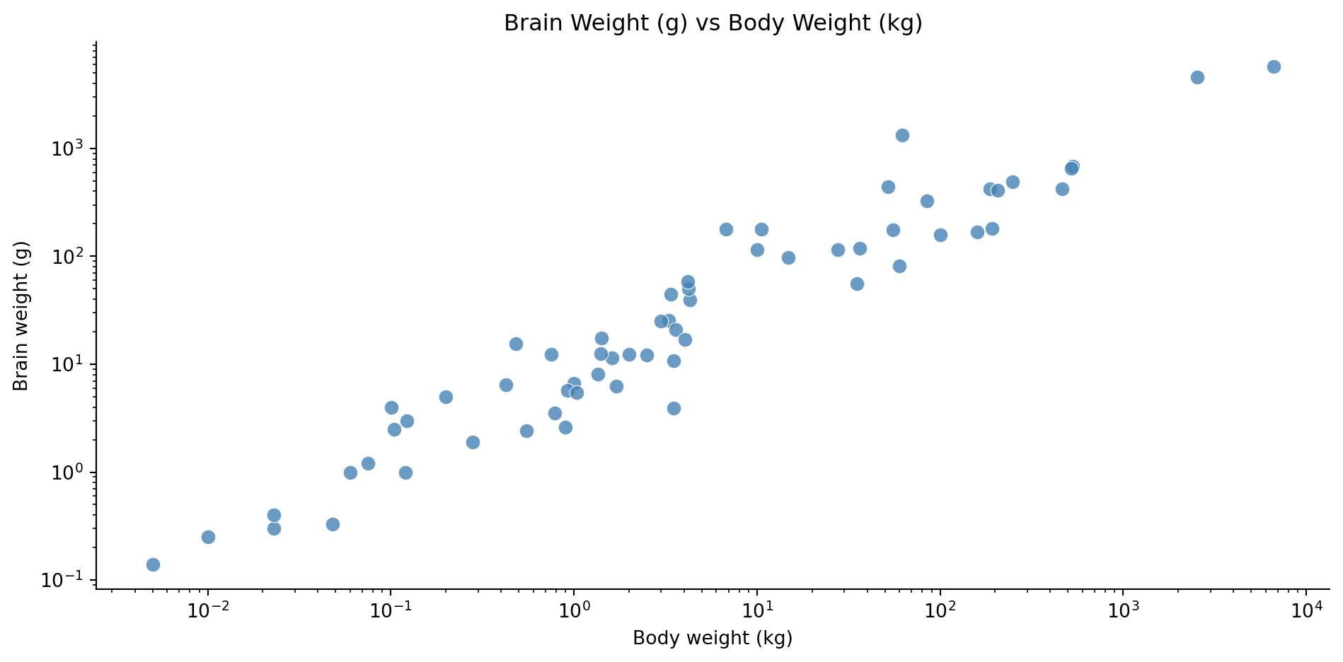
  • There is a clear linear relationship between the variables on the log scale.

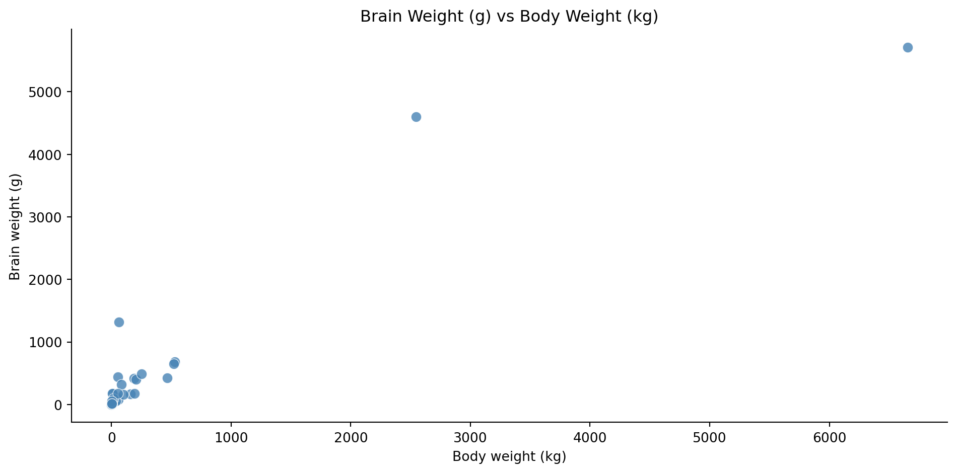
  • The plot shows a positive relationship between the variables.
  • To better see the relationship, we can use log-log axes.

DSL Example - Analyze

Linear Model

Our visualization suggests that the relationship could be modeled as

\[ \begin{aligned} \log(\text{brain}) & = \beta_0 + \beta_1 \log(\text{body})\\ \text{brain} & = \exp(\beta_0 + \beta_1 \log(\text{body})) \\ \text{brain} & = c\cdot\exp(\log(\text{body}^{\beta_1})) \\ \implies \text{brain} & \propto \text{body}^{\beta_1}. \end{aligned} \]

This suggests that the relationship is a power law.

  • To determine the parameters of the model, we can use linear regression.
    • We will discuss this in more detail later.
    • Let’s have a quick look at the fitted model details.

DSL Example - Model

                             OLS Regression Results                             
================================================================================
Dep. Variable:     np.log(brain_weight)   R-squared:                       0.921
Model:                              OLS   Adj. R-squared:                  0.919
Method:                   Least Squares   F-statistic:                     697.4
Date:                  Tue, 07 Apr 2026   Prob (F-statistic):           9.84e-35
Time:                          22:12:32   Log-Likelihood:                -64.336
No. Observations:                    62   AIC:                             132.7
Df Residuals:                        60   BIC:                             136.9
Df Model:                             1                                         
Covariance Type:              nonrobust                                         
=======================================================================================
                          coef    std err          t      P>|t|      [0.025      0.975]
---------------------------------------------------------------------------------------
Intercept               2.1348      0.096     22.227      0.000       1.943       2.327
np.log(body_weight)     0.7517      0.028     26.409      0.000       0.695       0.809
==============================================================================
Omnibus:                        2.698   Durbin-Watson:                   1.667
Prob(Omnibus):                  0.260   Jarque-Bera (JB):                1.933
Skew:                           0.405   Prob(JB):                        0.380
Kurtosis:                       3.301   Cond. No.                         3.73
==============================================================================

Notes:
[1] Standard Errors assume that the covariance matrix of the errors is correctly specified.
  • R-squared = 0.921 β€” \(\log(\text{body weight})\) explains 92.1% of the variance in \(\log(\text{brain weight})\).
  • F-statistic p-value = 9.84e-35 β€” the model is highly statistically significant overall.
  • Slope = 0.7517
    • p-values of 0.000, so highly significant.

DSL Example - Interpret

Our fitted model is:

\[ \text{brain} \propto \text{body}^{0.7517}. \]

  • This means that a 1% increase in body weight is associated with a ~0.75% increase in brain weight.

  • This leads us to draw the following conclusion:

For these 62 mammals there is evidence that brain weight changes in proportion to a power of body weight.

  • Note that this conclusion is not very strong since:
    • Data set is relatively small.
    • Not representative of mammals in general.
    • Aggregated data, not individual level.

Conclusion

Conclusion

βœ… What we covered

  • Course information.
  • What is data science?
    • Data and Datasets
    • Key terminology.
    • Data types.
  • The data science lifecycle.

πŸ“… What’s next?

  • Handling data in Python.
  • Data structure.
  • Data preparation.

References

Allison, T., and D. V. Cicchetti. 1976. β€œSleep in Mammals: Ecological and Constitutional Correlates.” Science 194 (4266): 732–34. https://doi.org/10.1126/science.982039.