PSTAT 10 Data Science Principles

Lecture 16: Aggregating and Joins

John Robin Inston

johninston@ucsb.edu

University of California, Santa Barbara

September 1, 2026

Introduction

🔁 Review: Lecture 15

👈 So far we have looked at:

• Database connections
• SELECT queries
• Aliases
• Aggregation (MAX, MIN, COUNT)

👀 Outline: Lecture 16

👇 Today we will look more closely at:

• Aggregation
• COUNT, SUM, AVERAGE, etc.
• Grouping

We will also look at Joins, specifically:

• Inner joins
• Left, right and full outer joins

Connecting

🔌 Chinook Database

For this lecture you will need the usual database connection. Make sure you have it set up now:

library(DBI)
library(RSQLite)
library(sqldf)

Create an appropriate database object:

chinook_db <- dbConnect(
    SQLite(),
    "data/Chinook_Sqlite.sqlite"
)

📌 As usual, if you do not have an appropriate file path pointing to the .sqlite file, R will populate an empty database object. If you wish to avoid working with file paths, place the .sqlite file in your current working directory.

🔍 Advanced Queries

All of our queries in previous lectures had something in common:

• They retrieved information from a single table!

SELECT [attributes] FROM [table] WHERE [logicals]

A simple query retrieves information from a single table.

A complex query searches for information across multiple tables.

To retrieve information across multiple tables, we will need to use joins.

• But first, we will look at aggregation and grouping.

Aggregation

➕ Basic Aggregation Functions — SUM

Aggregation functions collapse many rows into a single summary value. We have previously worked with COUNT, MIN and MAX.

• SUM returns the total of a numeric column.
• Here we sum every track length on album 154 (converted to minutes):

chinook_db |>
  dbGetQuery(
    "SELECT SUM(milliseconds)/60000 AS album_length_min
    FROM Track
    WHERE AlbumId = 154"
  )

  album_length_min
1               47

➗ Basic Aggregation Functions — AVG

We often want to find the average of a numeric column.

• AVG returns the mean of a numeric column.
• Here we take the average track length on album 154 (again in minutes):

chinook_db |>
  dbGetQuery(
    "SELECT AVG(milliseconds)/60000 AS avg_minutes
    FROM Track
    WHERE AlbumId = 154"
  )

  avg_minutes
1    5.938933

🎯 Motivating Aggregation

What if we wanted to find the average track length for each album with AlbumId between 150 and 155?

• We are not looking for the cumulative average.
• Our desired output looks something like this:

  AlbumId avg_minutes
1       1    4.000692
2       2    5.709367
3       3    4.767156
4       4    5.110956
5       5    4.901899

📊 Aggregation

Not quite right…

Directly using logicals we run into problems:

chinook_db |>
  dbGetQuery(
    "SELECT AlbumId,AVG(Milliseconds)/60000 
      AS avg_minutes
    FROM Track
    WHERE AlbumId >= 150 AND AlbumId <= 155")

  AlbumId avg_minutes
1     150    5.997313

📊 Aggregation — GROUP BY

We need to specify groups with GROUP BY:

chinook_db |>
  dbGetQuery(
    "SELECT AlbumId, AVG(Milliseconds)/60000 
      AS avg_minutes
    FROM Track GROUP BY AlbumId
    LIMIT 5"
  )

  AlbumId avg_minutes
1       1    4.000692
2       2    5.709367
3       3    4.767156
4       4    5.110956
5       5    4.901899

📊 Querying with Aggregation

Again, not quite right…

We can combine GROUP BY with WHERE clauses. However if we try just using WHERE we run into problems:

chinook_db |>
  dbGetQuery(
    "SELECT AlbumId, AVG(Milliseconds)/60000 
      AS avg_minutes
    FROM Track
    GROUP BY AlbumId
    WHERE AlbumId >= 150 AND AlbumId <= 155 ")

Error: near "WHERE": syntax error

📊 Querying with Aggregation — HAVING

We must use HAVING to declare clauses on aggregates:

chinook_db |>
  dbGetQuery(
    "SELECT AlbumId, AVG(Milliseconds)/60000 
      AS avg_minutes
    FROM Track GROUP BY AlbumId
    HAVING AlbumId BETWEEN 150 AND 155"
  )

  AlbumId avg_minutes
1     150    5.134753
2     151    5.641196
3     152    6.846198
4     153    5.854236
5     154    5.938933
6     155    6.828874

🧮 Example — Combined Aggregation

Suppose we wish to select AlbumId, alongside a column detailing the number of tracks on each album with AlbumId between 150 and 155.

chinook_db |>
  dbGetQuery(
    "SELECT AlbumId, COUNT(*)
    FROM Track GROUP BY AlbumId
    HAVING AlbumId >= 150 AND AlbumId <= 155"
  )

  AlbumId COUNT(*)
1     150       10
2     151       14
3     152        8
4     153       13
5     154        8
6     155       11

We can add appropriate aliasing for reader clarity when possible:

chinook_db |>
  dbGetQuery(
    "SELECT AlbumId, COUNT(*) as Track_Count
    FROM Track GROUP BY AlbumId
    HAVING AlbumId >= 150 AND AlbumId <= 155"
  )

  AlbumId Track_Count
1     150          10
2     151          14
3     152           8
4     153          13
5     154           8
6     155          11

⚖️ Combining WHERE and Aggregation

It is important to understand the structure of SQL queries with aggregation.

• WHERE is used when creating clauses applied on all data.
• WHERE cannot be combined with GROUP BY.
• GROUP BY combines all data corresponding to an appropriate clause.
• HAVING is used with queries on aggregate clauses.

📌 All of these tools can be combined in the same query.

⚖️ Example — Combining WHERE and Aggregation

Suppose we are interested in returning the AlbumId, and the Total_Price of all albums with MediaTypeId of 3 and AlbumId between 220 and 250:

chinook_db |>
  dbGetQuery(
    "SELECT AlbumId, SUM(UnitPrice) 
      AS Total_Price
    FROM Track 
    WHERE MediaTypeID = 3 
    GROUP BY AlbumId
    HAVING AlbumId BETWEEN 220 AND 250")

  AlbumId Total_Price
1     226        1.99
2     227       37.81
3     228       45.77
4     229       51.74
5     230       49.75
6     231       47.76
7     249       11.94
8     250       43.78

As soon as we add aggregation, we need to group the data appropriately. We can then use HAVING to filter on the grouped data.

📝 Query Organization

Recall our simple queries followed the structure:

SELECT [attribute] FROM [table] WHERE [clause]

• We can generalize the structure to include aggregates.
• We can also consider ordering.

# GENERAL SELECT QUERY
SELECT attributes
FROM relations
WHERE conditions
GROUP By attributes
HAVING conditions
ORDER BY attributes

💪 Exercise — Full Queries

05:00

Try to construct the query returning the AlbumId, GenreId, and length of each album in minutes as Album_Length (use scaled Milliseconds to compute, and use aliasing) of all albums with ID between 100 and 200 from the relation Track.

1. You will need to group the tracks by album.
2. Only select albums with GenreId of 3.
3. Order the results by album length (descending).
4. Return the first 10 rows of your query.

✅ Solution — Full Queries

chinook_db |>
  dbGetQuery(
    "SELECT AlbumId, GenreId, SUM(Milliseconds)/60000 as AlbumLength
    FROM Track WHERE GenreId = 3
    GROUP BY AlbumId
    HAVING AlbumId BETWEEN 100 AND 200
    ORDER BY AlbumLength DESC
    LIMIT 7"
  )

  AlbumId GenreId AlbumLength
1     151       3          78
2     153       3          76
3     155       3          75
4     162       3          73
5     174       3          72
6     149       3          70
7     141       3          68

Reading the query clause by clause:

• WHERE GenreId = 3 filters to the right genre before grouping.
• GROUP BY AlbumId collapses tracks so SUM gives one length per album.
• HAVING AlbumId BETWEEN 100 AND 200 filters on the grouped result.
• ORDER BY AlbumLength DESC then LIMIT 7 return the longest albums first.

Joins

🔗 Limits of Simple Queries

Know your limitations

• Our queries have gotten progressively more complex, but they have still only involved a single table (usually Track).
• This simplified query structure is useful, but insufficient for relational databases.
• Remember we split related data across tables.

For example, what if we want the album name? There is no such attribute in Track!

chinook_db |>
  dbGetQuery(
    "SELECT TrackId, Name, AlbumId
    FROM Track
    WHERE AlbumId = 194 LIMIT 5"
  )

🔗 Querying Across Tables

I will prove it to you:

dbListFields(chinook_db, "track")

[1] "TrackId"      "Name"         "AlbumId"      "MediaTypeId"  "GenreId"     
[6] "Composer"     "Milliseconds" "Bytes"        "UnitPrice"   

You see! Album titles do appear in Album though:

dbListFields(chinook_db, "album")

[1] "AlbumId"  "Title"    "ArtistId"

🔗 Naive Approach

Step 1:

Query tracks:

chinook_db |>
  dbGetQuery(
    "SELECT TrackId, Name, AlbumId
    FROM Track WHERE AlbumId = 194
    LIMIT 10"
  )

   TrackId                       Name AlbumId
1     2375                 By The Way     194
2     2376       Universally Speaking     194
3     2377          This Is The Place     194
4     2378                      Dosed     194
5     2379            Don't Forget Me     194
6     2380            The Zephyr Song     194
7     2381                 Can't Stop     194
8     2382        I Could Die For You     194
9     2383                   Midnight     194
10    2384 Throw Away Your Television     194

Step 2

Query albums:

chinook_db |>
  dbGetQuery(
    "SELECT *
    FROM Album
    WHERE AlbumId = 194"
  )

  AlbumId      Title ArtistId
1     194 By The Way      127

😭 There has to be a better way!!

🕸️ Structure

Relation Structure

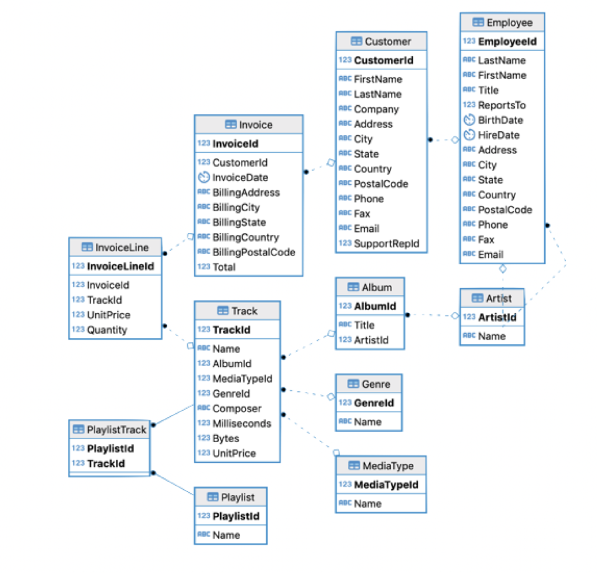
• Each box is a table; each arrow links a foreign key to the primary key it references.
• To pull Track and Album info together, we follow the arrow on AlbumId.

🔗 Better Approach: Joins

Recall the structure of relational databases from lectures 13-15:

• AlbumId is the primary key in Album.
• AlbumId is the foreign key in Track corresponding to AlbumId in Album.
• To combine inputs, we will JOIN on the keys!

# INNER JOIN
chinook_db |>
  dbGetQuery(
    "SELECT TrackId, Name, Track.AlbumId, Title
    FROM Track 
    INNER JOIN Album ON Track.AlbumId = Album.AlbumId
    WHERE Track.AlbumId = 194 
    LIMIT 3")

  TrackId                 Name AlbumId      Title
1    2375           By The Way     194 By The Way
2    2376 Universally Speaking     194 By The Way
3    2377    This Is The Place     194 By The Way

🔗 Inner Join Syntax

Inner join structure is as follows:

[Table 1] INNER JOIN [Table 2] ON [key1] = [key2]

• Note that we need to specify Track.AlbumId and Album.AlbumId.
• The Table.Attribute syntax is used when identically named attributes exist in multiple tables.
• SQL will not know what you mean by default.
• It is common to use aliases in these queries.

💪 Exercise — Aggregation and Joins

05:00

Write a single query that does the following:

1. Returns the average length of tracks in each genre in seconds, in a column called GenreAvg.
2. Returns the name of each corresponding genre.

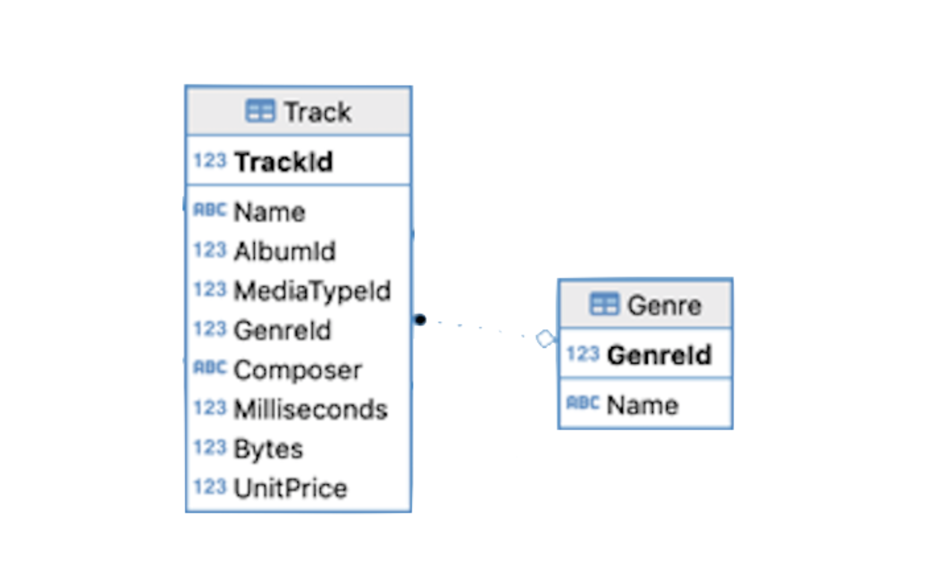
📌 Hint 1: You will need to join the Track and Genre tables. Hint 2: You will need to group by GenreId.

✅ Solution — Aggregation and Joins

chinook_db |>
  dbGetQuery(
    "SELECT AVG(Milliseconds)/60000 AS GenreAvg, g.Name
    FROM Track t 
    JOIN Genre g ON t.GenreId = g.GenreId
    GROUP BY t.GenreId 
    LIMIT 3")

  GenreAvg  Name
1 4.731834  Rock
2 4.862590  Jazz
3 5.162491 Metal

• JOIN can directly replace INNER JOIN.
• We can make joins less cumbersome with aliases.

📌 Make sure you understand how aliases were used here — this format will appear throughout assignments.

🔗 No Key Specification

We can also join tables without specifying the key to join on.

The Cartesian product of two tables returns every combination of records in both tables.

chinook_db |>
  dbGetQuery(
    "SELECT al.Title, al.ArtistId, ar.ArtistId, ar.Name
    FROM Album al 
    JOIN Artist ar LIMIT 3")

                                  Title ArtistId ArtistId      Name
1 For Those About To Rock We Salute You        1        1     AC/DC
2 For Those About To Rock We Salute You        1        2    Accept
3 For Those About To Rock We Salute You        1        3 Aerosmith

• We usually do not want to do this! — it produces a huge, mostly meaningless table.
• Similar functionality exists using CROSS JOIN.

🔗 Implicit Joins

We can effectively construct an inner join using the Cartesian product:

• Join tables together using an inner join.
• Use WHERE clauses to select appropriate attributes.

chinook_db |>
  dbGetQuery(
    "SELECT al.Title, al.ArtistId, ar.ArtistId, ar.Name
    FROM Album al 
    JOIN Artist ar
    WHERE al.ArtistID = ar.ArtistID LIMIT 2")

                                  Title ArtistId ArtistId   Name
1 For Those About To Rock We Salute You        1        1  AC/DC
2                     Balls to the Wall        2        2 Accept

An implicit join constructs an inner join from the Cartesian product by adding a WHERE clause on the keys.

📌 Do not use this technique! Specify your joins explicitly.

🔑 Foreign and Primary Key Alignment

Foreign keys and primary keys.

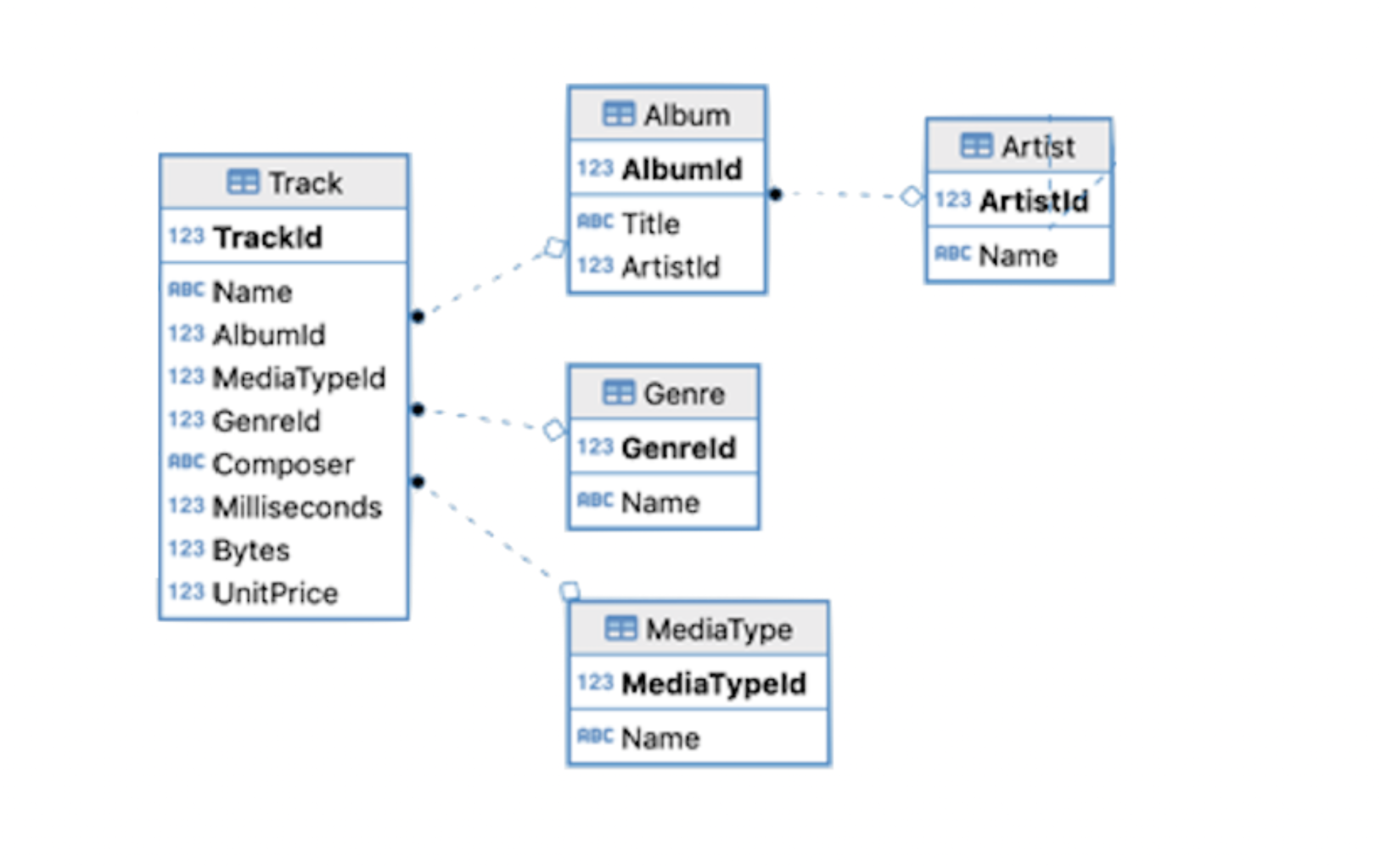
Note that foreign key names often match primary key names:

• AlbumId is foreign key in Track, primary key in Album.
• GenreId is foreign key in Track, primary key in Genre.
• ArtistId is foreign key in Album, primary key in Artist.

🔗 Natural Joins

When foreign and primary key names align, NATURAL JOIN can be used.

chinook_db |>
  dbGetQuery(
    "SELECT * FROM Album 
    NATURAL JOIN Artist 
    LIMIT 5"
  )

  AlbumId                                 Title ArtistId      Name
1       1 For Those About To Rock We Salute You        1     AC/DC
2       2                     Balls to the Wall        2    Accept
3       3                     Restless and Wild        2    Accept
4       4                     Let There Be Rock        1     AC/DC
5       5                              Big Ones        3 Aerosmith

• The one case where SQL infers the appropriate keys.
• Natural joins need to be used with extreme care.

🔗 Understanding Natural Joins

What is happening here?

chinook_db |>
  dbGetQuery(
    "SELECT TrackId, Name, MediaTypeId 
    FROM Track 
    NATURAL JOIN MediaType")

[1] TrackId     Name        MediaTypeId
<0 rows> (or 0-length row.names)

• Name appears in both Track and MediaType.
• Name corresponds to a different thing in each table.
• SQL does not know what to do.

📌 If you use natural joins, you need to be extremely careful — use explicit joins!

🔗 Inner Join

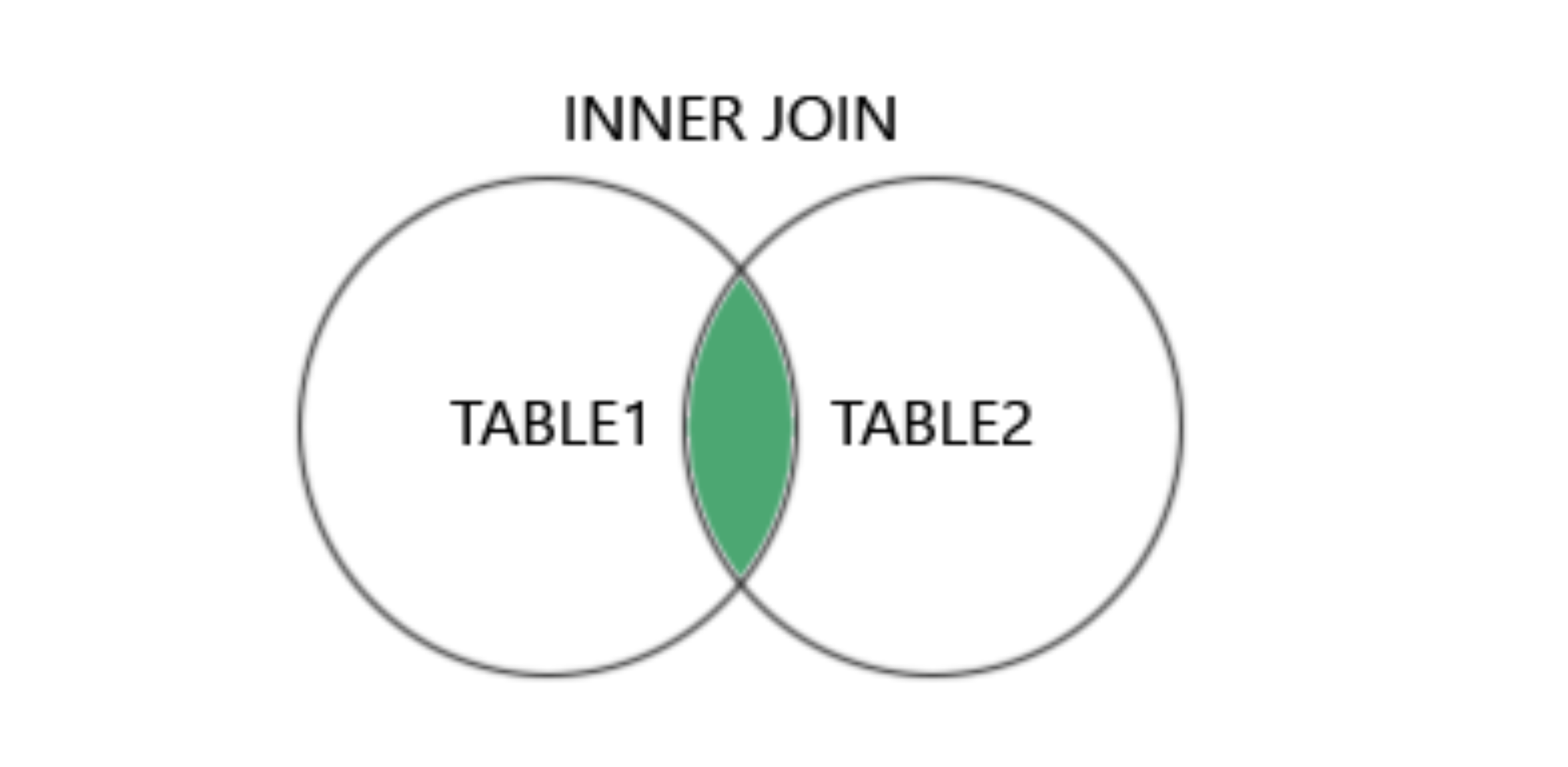
So far every join we have seen is an inner join — it keeps only rows with a match in both tables.

Inner Join

🔗 Motivating Outer Joins

• Inner joins combine matching attributes across tables.
• We have inner-joined matching ArtistId and AlbumId values.
• This is the most common type of join, and the main type used in PSTAT 10.

Suppose we add a track to the database. Let’s add “Cardigan”:

dbExecute(
  chinook_db,
  "INSERT INTO Track (TrackId, Name, AlbumId, MediaTypeId,
    Composer, Milliseconds,UnitPrice)
  VALUES (9995, 'Cardigan', 999, 1,
    'Taylor Swift', 239000, 0.99)"
)

🔗 Limitations of Inner Joins

We want to join this song to its album. Using an inner join gets us nowhere:

chinook_db |>
  dbGetQuery(
    "SELECT t.TrackId, t.Name,
    t.AlbumId, a.Title
    FROM Track t
    INNER JOIN Album a ON t.AlbumId = a.AlbumId
    WHERE t.TrackId = 9995"
  )

[1] TrackId Name    AlbumId Title  
<0 rows> (or 0-length row.names)

🔗 Outer Joins

A left outer join solves the problem:

chinook_db |>
  dbGetQuery(
    "SELECT t.TrackId, t.Name,
    t.AlbumId, a.Title
    FROM Track t
    LEFT JOIN Album a ON t.AlbumId = a.AlbumId
    WHERE t.TrackId = 9995"
  )

  TrackId     Name AlbumId Title
1    9995 Cardigan     999  <NA>

• What is happening here?
  • The left join keeps all rows from the left table (Track), and matches rows from the right table (Album) where possible.

🔗 Left and Right Outer Joins

Left and Right Joints

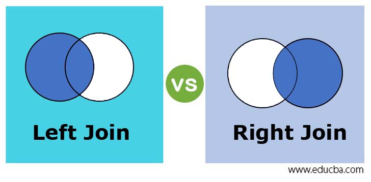
• Left and right joins function similarly.
• Each joins the intersection of T1 and T2 with the remainder of the (left/right) table.

🔗 Full Outer Joins

Full outer join.

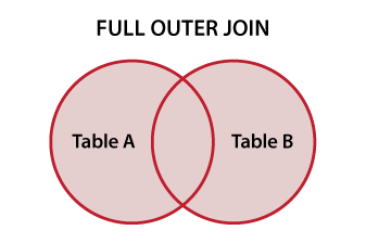
• Full outer joins complete the trifecta.
• They return the complete union between both tables — every row from both sides, matched where possible.

Summary

✅ Topics Covered

🤔 This lecture covered aggregation and joins, including:

• GROUP BY command
• WHERE versus HAVING
• Inner and natural joins
• Left, right, and full outer joins

📅 Next Class

🤩 Next class we will look at:

• How to modify database contents
• Database design
• Exercises with aggregation and joins