PSTAT 10 Data Science Principles

Lecture 14: SQL Queries

John Robin Inston

johninston@ucsb.edu

University of California, Santa Barbara

September 1, 2026

Introduction

🔁 Review: Lecture 13

👈 Last lecture we looked at databases, specifically:

• Relational Databases
• Data structure
  • Terminology (relations, tuples, domains, attributes)
  • Super, candidate, primary and foreign keys
• Data integrity

Also recall the following topics:

• The tidyverse library
• The pipe |> operator

👀 Outline: Lecture 14

👇 Today we will cover the following material:

• Preliminaries
  • The relational model
  • Structured Query Language (SQL)
• Core Pieces
  • Database engines (SQLite)
  • Interfacing databases in R
  • SQL Queries

Data Manipulation

🔁 Recap — Relational Model

Last lecture we discussed the relational model.

• We emphasized data structure (relations, keys, etc.).
• We discussed data integrity.
• We did not discuss the third piece: data manipulation.

Data manipulation is a slight misnomer — manipulating data could mean many things.

• Defining new database schema
• Searching for data within schema objects
• Controlling use permissions

📝 Structured Query Language (SQL)

SQL Programming Language

SQL is the most common language used in storing, querying and manipulating structured data.

• Data Definition Language (DDL) — define database schema
• Data Manipulation Language (DML) — add, modify or delete data
• Data Query Language (DQL) — retrieves data

📝 DCL & TCL

SQL Programming Language

Note that in PSTAT 10 we will not cover:

• Data Control Language (DCL) — manages access permissions (e.g. GRANT, REVOKE).
• Transaction Control Language (TCL) — manages transactions (e.g. COMMIT, ROLLBACK).

📌 These matter for multi-user, production databases — beyond our scope, where a single analyst queries a local database.

⚙️ Database Engines and SQLite

SQLite Software

The database engine is the software a DBMS uses to interface with its contents.

• It is not a database itself.
• We will use the SQLite database engine.
• SQLite is the most widely used database engine worldwide.
• Phones, computers, televisions, etc. all use SQLite.

🔌 Databases and R

To interface with databases using R we will use RSQLite.

• RSQLite embeds SQLite in R.
• This grants us access to the SQLite functionality with an R interface.
• We also install some additional helpful database packages.

# Package installation (do not include in documents)
install.packages("RSQLite")
install.packages("DBI") # database interface
install.packages("sqldf") # SQL dataframe

📦 Database Packages

Load the required packages by running the code below:

library(RSQLite)
library(DBI)
library(sqldf)

• RSQLite allows us to interface with DBs using SQL code in R.
• DBI constructs the database interface.
• sqldf allows us to manipulate R data frames using SQL.

📌 If you do not have all three libraries loaded, code appearing later in the lecture will break.

Tiny Clothes Database

💪 Exercise — Loading the Database

02:00

Our initial database work in this course uses the TinyClothesDB.

• This database contains the orders of a small online clothing store.
• It stores customer, product and sales information.
• Our first step is to establish a connection to the database.

Download the tc_clean.sqlite file from Canvas and put it in your current working directory.

🔌 Database Connections

To access the database, we need to create a connection to the database file. We do so using the dbConnect() function:

dbConnect(SQLite(), "path_to_my_db/my_db.sqlite")

Since we store our data in a separate data folder, our function is:

dbConnect(SQLite(), "data/tc_clean.sqlite")

🔌 Database Connection Object

We cannot interface with the database using the <SQLiteConnection> directly. We must save it as an object.

tc_db <- dbConnect(SQLite(),"data/tc_clean.sqlite")

We now have all the pieces we need:

• Our database connection tc_db
• SQL and database interfaces (DBI, RSQLite, sqldf)

🔍 Exploring Databases

A dbConnect object only lets us interface with the database.

• It tells us nothing about its structure.
• A useful first step (especially for a small database) is to explore it.

The dbListTables() function returns the relation names in the remote database.

dbListTables(database_connection_object)

The dbListFields() function returns the field names of a remote relation.

dbListFields(database_connection_object, "table")

🔍 Tiny Clothes Database — dbListTables()

We apply the dbListTables() and dbListFields() functions to our tc_db connection object.

dbListTables(tc_db)

[1] "Customer"       "Product"        "SalesOrder"     "SalesOrderLine"

We see our database has four tables:

• Customer
• Product
• SalesOrder
• SalesOrderLine

🔍 Tiny Clothes Database — dbListFields()

dbListFields(tc_db, "Customer")

[1] "CustomerId" "Name"       "Address"   

The attributes of the relation of interest are:

• CustomerId
• Name
• Address

📌 In general these functions become less useful as database and relation size increases!

💪 Exercise — Database Exploration

03:00

Use the dbListFields() command to determine the attributes of the Product, SalesOrder and SalesOrderLine tables.

• As you go through, think: which attributes could make up primary keys for each table?
• Which attributes could be foreign keys linking tables?

✅ Solution — Database Exploration

dbListFields(tc_db, "Product")
dbListFields(tc_db, "SalesOrder")
dbListFields(tc_db, "SalesOrderLine")

[1] "ProductId" "Name"      "Color"    

[1] "CustomerId" "OrderId"    "Date"      

[1] "OrderId"   "ProductId" "Quantity" 

Likely primary keys — the Id attribute that uniquely identifies each row:

• ProductId for Product, OrderId for SalesOrder, SalesOrderLineId for SalesOrderLine.

Likely foreign keys — attributes that point to another table’s primary key:

• SalesOrder holds a CustomerId → links each order to the Customer who placed it.
• SalesOrderLine holds an OrderId and a ProductId → links each line to its SalesOrder and to the Product sold.

🔑 Accessing Table Attributes

So far, we have functions to:

• Identify all database tables
• Identify header attributes of any table

The next step is actually accessing table data, which will require us to write our first SQL query:

• Everything we’ve done so far is just R.
• Both dbListTables() and dbListFields() are just R functions.

📝 SQL Query Structure

Basic SQL query structure is detailed below:

SELECT attributes
FROM relations
WHERE conditions

For example, the following query would return the ProductId and Name columns from all rows of Product where ProductId > 1:

SELECT ProductId, Name FROM Product WHERE ProductId > 1

Error: <text>:1:8: unexpected symbol
1: SELECT ProductId
           ^

📌 R cannot interpret SQL code directly.

📝 Interpreting SQL

dbGetQuery(database_connection_object, SQL_query)
dbExecute(database_connection_object, SQL_query)

To work with SQL queries in R, we can use the functions dbGetQuery() and dbExecute() from the DBI library.

• Use dbGetQuery() for SELECT queries only.
• dbGetQuery() returns the query result as an R dataframe.
• Queries that alter database tables use dbExecute().

📌 dbGetQuery() may ostensibly work with commands that should use dbExecute(), but you can very quickly run into errors and compatibility issues.

📝 Example — Running SQL Queries

Let’s consider our previous query, which returned the ProductId and Name columns from all rows of Product where ProductId > 1.

Using the query as an argument in the dbGetQuery() command yields the result of interest.

dbGetQuery(tc_db,
          "SELECT ProductId, Name
           FROM Product
           WHERE ProductId > 1")

  ProductId   Name
1         2  Pants
2         3  Socks
3         4  Socks
4         5 Shirts

💪 Exercise — Basic Queries

05:00

SELECT queries are the bread and butter of SQL! You’re going to be writing several of them in the next few assignments, so write two for practice now.

1. Write and execute a query to return a dataframe containing the CustomerId, Name and Address values of all customers whose addresses are either "State" or "Ocean".
2. Write and execute a query to return the Date values of all sales orders where OrderId is greater than 5.

✅ Solution — Basic Queries

dbGetQuery(tc_db,
          "SELECT CustomerId, Name, Address
           FROM Customer
           WHERE Address = 'State' or Address = 'Ocean'")
dbGetQuery(tc_db,
          "SELECT Date
           FROM SalesOrder
           WHERE OrderId > 5")

  CustomerId  Name Address
1          1  Alex   State
2          3 Carol   Ocean

      Date
1  8/16/19
2 10/12/19

Reading each query as SELECT (columns) FROM (table) WHERE (condition):

• Query 1 selects three columns from Customer; the WHERE uses or so a row qualifies if Address is 'State' or 'Ocean'.
• Query 2 selects only Date from SalesOrder; the WHERE keeps rows where the OrderId > 5 comparison is true.

🔄 Improving Queries

Our queries so far have been very basic — we are working with a very basic database.

Let’s see how queries translate to a much more complex database.

Before connecting to the new database, close the old connection using the code below.

dbDisconnect(tc_db) # no outputs; closes database connection

Chinook Database

🎸 Chinook Database

For the remaining exercises we will use the Chinook database. This database is a useful training tool for several reasons:

• It is fairly complex, as it consists of 11 interconnected relations.
• The structural complexities discussed in previous lectures are on full display.
• The database contains lots of data; its tables span thousands of tuples.

Download the Chinook_Sqlite.sqlite file from Canvas. Put it in your working directory.

Save it to an object using the code below.

chinook_db <- dbConnect(SQLite(), "data/Chinook_Sqlite.sqlite")

🔍 Exploring Complex Databases

Exploring tables is usually an appropriate first step.

dbListTables(chinook_db)

 [1] "Album"         "Artist"        "Customer"      "Employee"     
 [5] "Genre"         "Invoice"       "InvoiceLine"   "MediaType"    
 [9] "Playlist"      "PlaylistTrack" "Track"        

Several of these tables are much larger than those in tc_db.

dbListFields(chinook_db, "Customer")

 [1] "CustomerId"   "FirstName"    "LastName"     "Company"      "Address"     
 [6] "City"         "State"        "Country"      "PostalCode"   "Phone"       
[11] "Fax"          "Email"        "SupportRepId"

📊 More than Dataframes

Running a SQL query through dbGetQuery() returns a dataframe:

dbGetQuery(
    chinook_db,
    "SELECT CustomerId, FirstName, LastName, Country
    FROM customer
    LIMIT 5"
)

  CustomerId FirstName    LastName        Country
1          1      Luís   Gonçalves         Brazil
2          2    Leonie      Köhler        Germany
3          3  François    Tremblay         Canada
4          4     Bjørn      Hansen         Norway
5          5 František Wichterlová Czech Republic

📌 The LIMIT argument functions similarly to the second argument of head() in R.

⚙️ PRAGMA Command

The PRAGMA command is a special tool for SQLite.

It is an SQL extension specific to SQLite and used to:

1. Modify the operation of the SQLite library; or
2. Query the SQLite library for internal (non-table) data.

📌 Queries with PRAGMA can get quite complex!

We will mainly work with:

• PRAGMA table_info(table)
• PRAGMA foreign_key_list(table)

⚙️ Example — PRAGMA Command

dbGetQuery(chinook_db,
          "PRAGMA table_info(Customer)")

   cid         name         type notnull dflt_value pk
1    0   CustomerId      INTEGER       1         NA  1
2    1    FirstName NVARCHAR(40)       1         NA  0
3    2     LastName NVARCHAR(20)       1         NA  0
4    3      Company NVARCHAR(80)       0         NA  0
5    4      Address NVARCHAR(70)       0         NA  0
6    5         City NVARCHAR(40)       0         NA  0
7    6        State NVARCHAR(40)       0         NA  0
8    7      Country NVARCHAR(40)       0         NA  0
9    8   PostalCode NVARCHAR(10)       0         NA  0
10   9        Phone NVARCHAR(24)       0         NA  0
11  10          Fax NVARCHAR(24)       0         NA  0
12  11        Email NVARCHAR(60)       1         NA  0
13  12 SupportRepId      INTEGER       0         NA  0

dbGetQuery(chinook_db,
          "PRAGMA foreign_key_list(Customer)")

  id seq    table         from         to on_update on_delete match
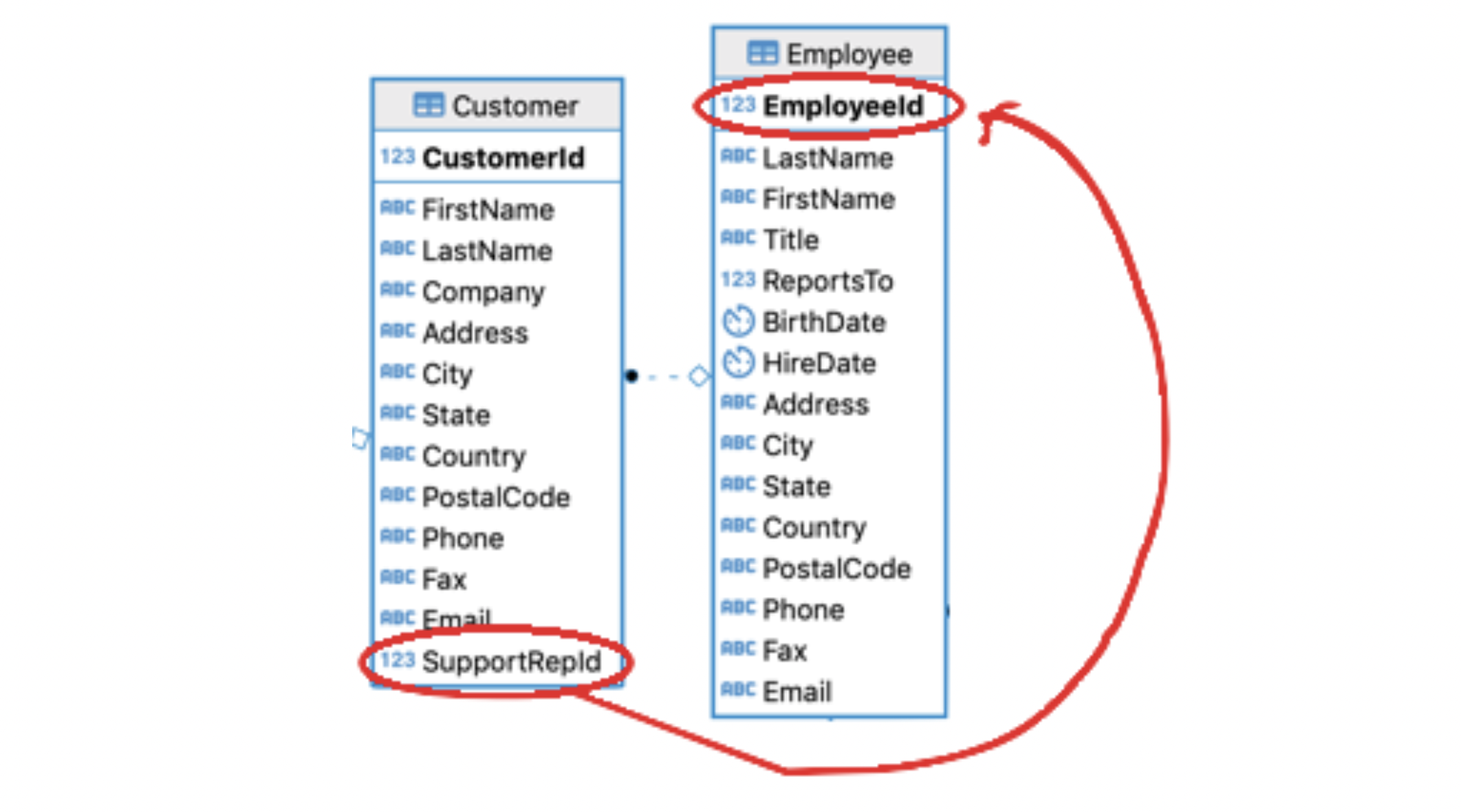
1  0   0 Employee SupportRepId EmployeeId NO ACTION NO ACTION  NONE

📌 Remember that a foreign key points to the primary key of another table.

Here SupportRepId in Customer points to EmployeeId in Employee.

🔑 foreign_key_list()

PRAGMA foreign_key_list(table) lists every foreign key defined on a relation.

• Each row is one foreign key on the queried table.
• from is the attribute in this table that acts as the foreign key.
• table and to name the relation and attribute it points to.

dbGetQuery(chinook_db,
          "PRAGMA foreign_key_list(Customer)")

  id seq    table         from         to on_update on_delete match
1  0   0 Employee SupportRepId EmployeeId NO ACTION NO ACTION  NONE

Understanding foreign keys.

🗄️ Dataframe Structure

Chinook relation network

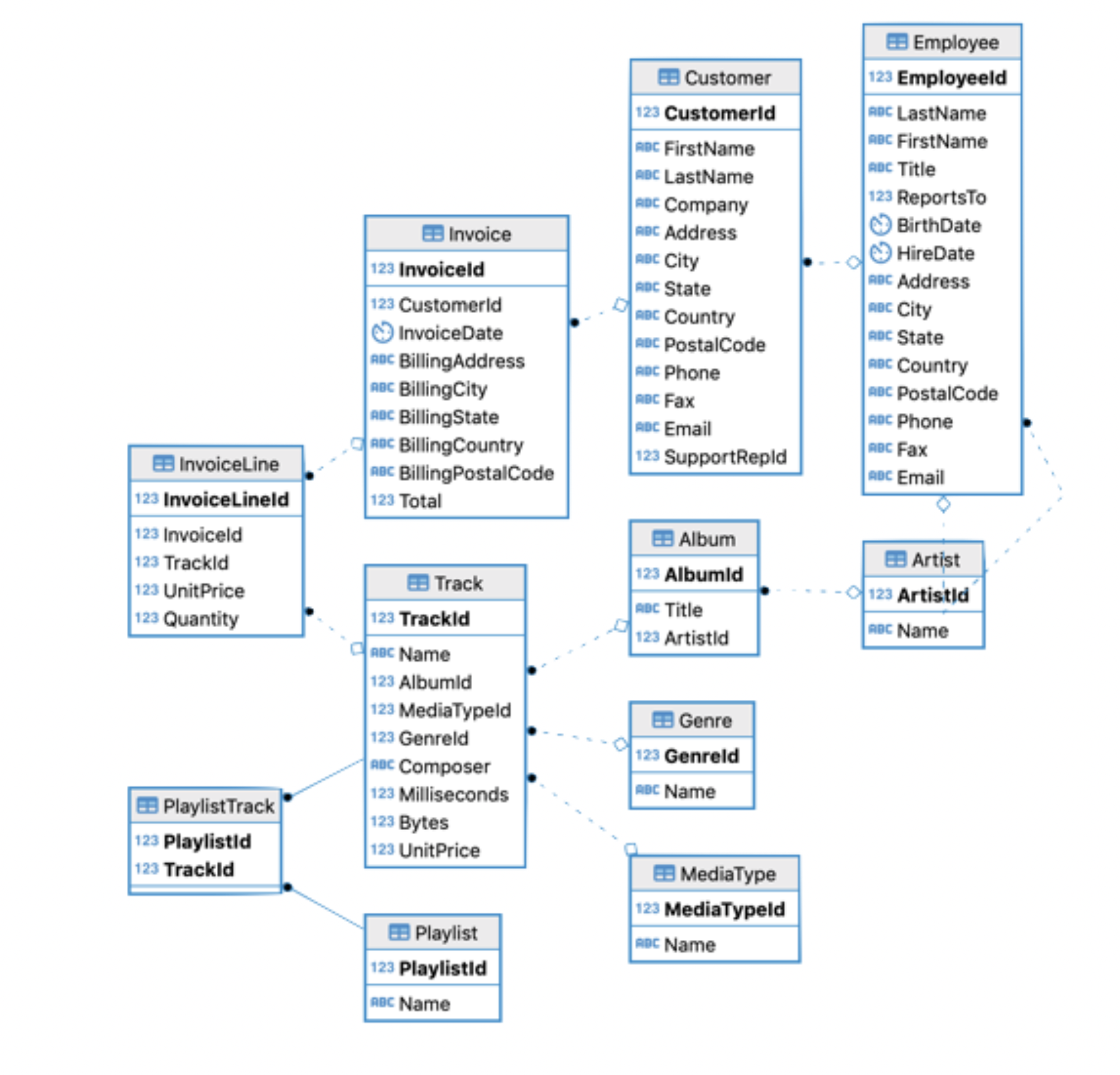
This diagram shows the same relationships that foreign_key_list() reported, but for the whole database at once.

• Each box is a relation; each arrow is a foreign key pointing to another table’s primary key.
• The 11 tables are interconnected — few tables stand alone.
• Reading these links is what lets us join tables together in later queries.

🔒 Data Integrity in Practice

So far we have only worked with SELECT (i.e. DQL queries). We can use INSERT to add to a table. This is a modification to the table, so we use dbExecute().

dbExecute(chinook_db,
          "INSERT INTO Customer (CustomerId, FirstName, LastName, Email)
          VALUES (97, 'John', 'Inston', 'johninston@ucsb.edu')")
dbGetQuery(chinook_db,
           "SELECT CustomerId,  FirstName, LastName, Email
           FROM Customer
           WHERE CustomerId = 97")

[1] 1

  CustomerId FirstName LastName               Email
1         97      John   Inston johninston@ucsb.edu

🔒 Data Integrity — Table Modification

We must satisfy entity integrity when modifying tables.

• Recall that primary key values must be unique.

dbExecute(chinook_db,
          "INSERT INTO Customer (CustomerId, FirstName, LastName, Email)
          VALUES (97, 'Blythe', 'King', 'blytheking@pstat.ucsb.edu')")

Error: UNIQUE constraint failed: Customer.CustomerId

📌 Note that SQLite allows NULL primary key values, violating entity integrity.

dbExecute(chinook_db,
          "INSERT INTO Customer (CustomerId, FirstName, LastName, Email)
          VALUES (NULL, 'Blythe', 'King', 'blytheking@pstat.ucsb.edu')")

🔗 Referential Integrity in Practice

We must also satisfy referential integrity when modifying tables.

• Recall that foreign keys must either point to an existing value or be NULL.
• SupportRepId is the Customer foreign key for EmployeeId.
• Referential integrity is not enforced by default.

dbExecute(chinook_db,
          "INSERT INTO Customer (CustomerId, FirstName, LastName, Email, SupportRepId)
          VALUES (92, 'Blythe', 'King', 'blytheking@pstat.ucsb.edu', 16384)")
dbExecute(chinook_db,
          "INSERT INTO Customer (CustomerId, FirstName, LastName, Email, SupportRepId)
          VALUES (90, 'Blythe', 'King', 'blytheking@pstat.ucsb.edu', 16384)")

[1] 1

[1] 1

🧹 Cleaning Up the Mess

Let’s look at what we have added to our database.

dbGetQuery(
    chinook_db,
    "SELECT CustomerId, FirstName, LastName, Email
    FROM Customer
    WHERE FirstName = 'Blythe' OR LastName = 'Inston'"
)

  CustomerId FirstName LastName                     Email
1         90    Blythe     King blytheking@pstat.ucsb.edu
2         92    Blythe     King blytheking@pstat.ucsb.edu
3         97      John   Inston       johninston@ucsb.edu

⚠️ DELETE Syntax

📌 Be very careful if you decide to use the DELETE syntax, as it does not allow you to undo mistakes and you will have to re-download the database.

In our case we delete the individuals that we added using the following code (you do not need to run this):

dbExecute(chinook_db,
  "DELETE FROM Customer
   WHERE FirstName = 'Blythe' OR LastName = 'Inston'")

[1] 3

✅ Final Checks

We perform a final check to ensure that we have left the database as we started:

dbGetQuery(
    chinook_db,
    "SELECT CustomerId, FirstName, LastName, Email
    FROM Customer
    WHERE FirstName = 'Blythe' OR LastName = 'Inston'"
)

[1] CustomerId FirstName  LastName   Email     
<0 rows> (or 0-length row.names)

📁 Wrapping Up

For the next few lectures, you should be thinking about organization.

• It is very easy to run into issues with database connections.
• Keep your database connection file somewhere logical.
• Close your connections after use!

dbDisconnect(chinook_db)

Summary

✅ Topics Covered

🤔 Today we looked at:

• Data Manipulation
• Tiny Clothes Database; and
• Chinook Database

📅 Next Class

🤩 Next class we will continue our exploration of databases and SQL with:

• Complex data selection
• SQL functions
• SQL syntax and convention

📌 Next lecture is code / syntax heavy, similar to early R lectures!