PSTAT 10 Data Science Principles

Lecture 12: Advanced Simulation

John Robin Inston

johninston@ucsb.edu

University of California, Santa Barbara

August 22, 2026

Introduction

🔁 Review: Lecture 11

👈 Last lecture we had yet another very math heavy lecture covering:

• Poisson Distributions
• Generalizing R Functions
• Continuous Random Variables
• Continuous Uniform Distribution
• Normal (Gaussian) Distribution

👀 Outline: Lecture 12

👇 This lecture we will conclude our study of probability by looking at:

• Simulation
• Harder probability questions
• Monte Carlo methods

📌 This will be our last R-focused lecture until Lecture 19, but R will still appear in homework and section exercises.

Simulating Pi

🥧 History of Estimating \(\pi\)

One of the oldest approximation problems humans have been working on is estimating \(\pi\).

There is evidence of estimating \(\pi\) as far back as:

• Ancient Babylon and Egypt (1700 - 1600 BCE)
• Ancient India (600 BCE)
• Ancient Greece (300 BCE)
• Ancient China (250 CE)

More recently we have estimated \(\pi\) using:

• Infinite series and trigonometric identities (middle ages)
• Rapidly converging infinite series (19th & 20th centuries)
• Supercomputers (modern day)

Estimating Pi.

🥧 Estimating Pi

Proposed Methodology

We attempt to construct our own estimate of \(\pi\) using simulation on the unit circle.

Area of a Circle

Recall from basic trigonometry that the area of a circle is given by:

\[ A = \pi \times r^2. \]

When considering a unit circle \(r=1\), and so

\[ A = \pi. \]

Hence if we can approximate the area of a unit circle we approximate \(\pi\).

🥧 Approximate Unit Circle Area

Step by Step Approach

To approximate the area of the unit circle our approach is as follows:

1. Draw a unit circle.
2. Enclose the unit circle perfectly in a unit square.
3. Simulate points uniformly in the square.
4. Determine the proportion of points that land within the unit circle.
5. This proportion is an approximation of the area of the circle \(\pi\) over the area of the square \(4\), and so we compute:

\[ \pi \approx 4 \times \text{Prop} \]

⭕ Draw a Circle

We draw a circle!

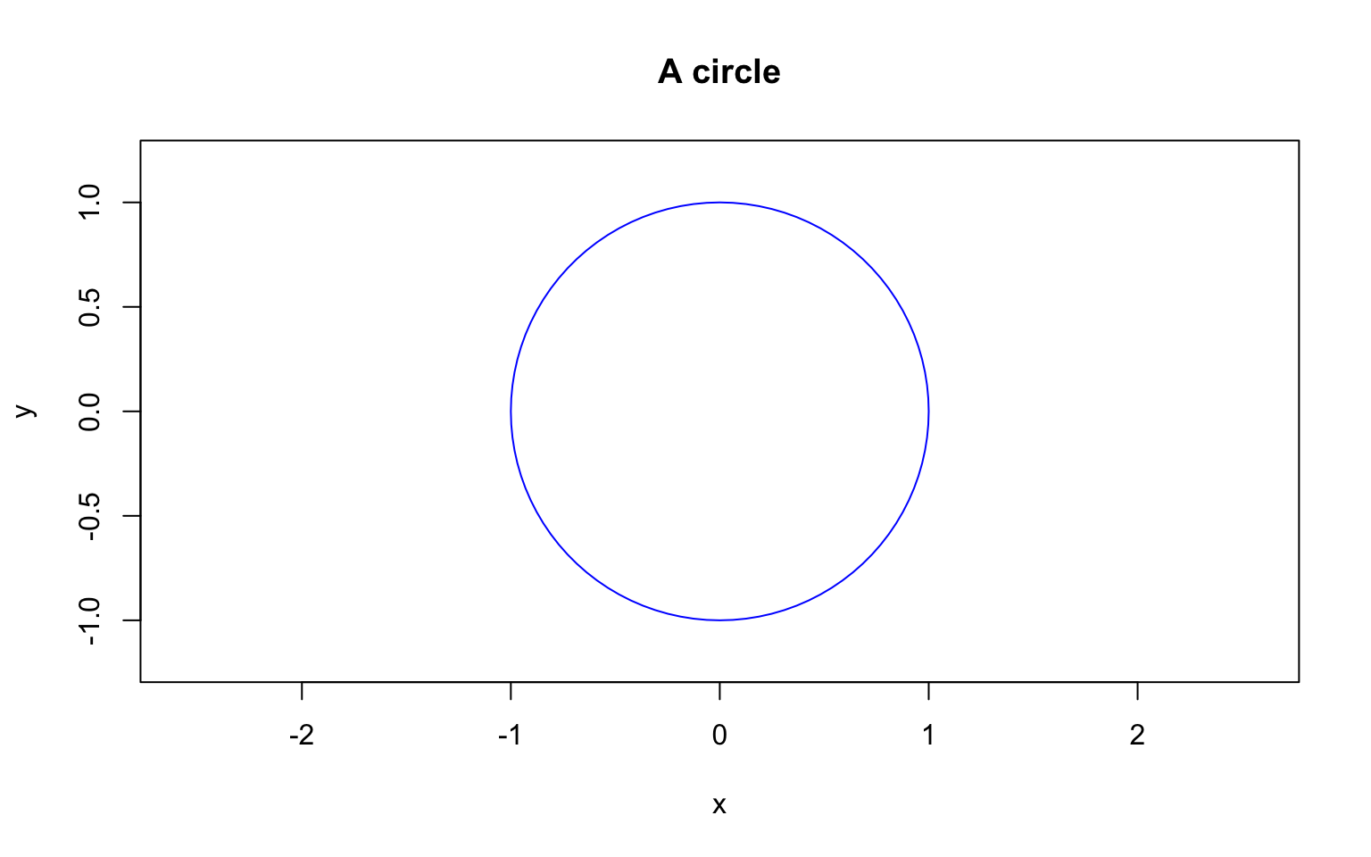
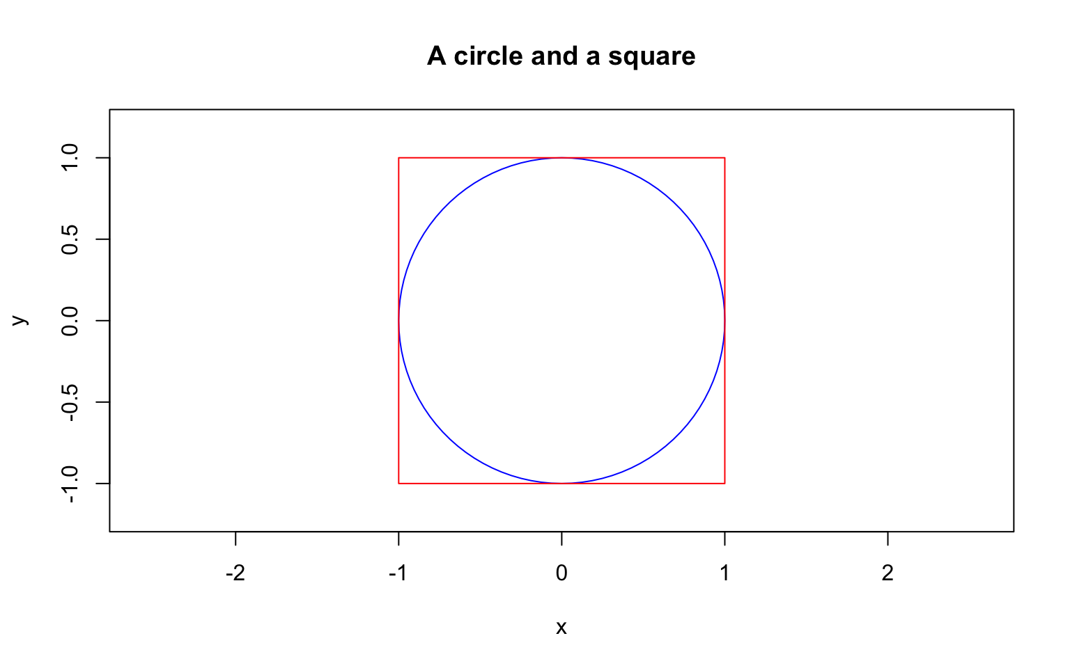
⬜ Draw a Square

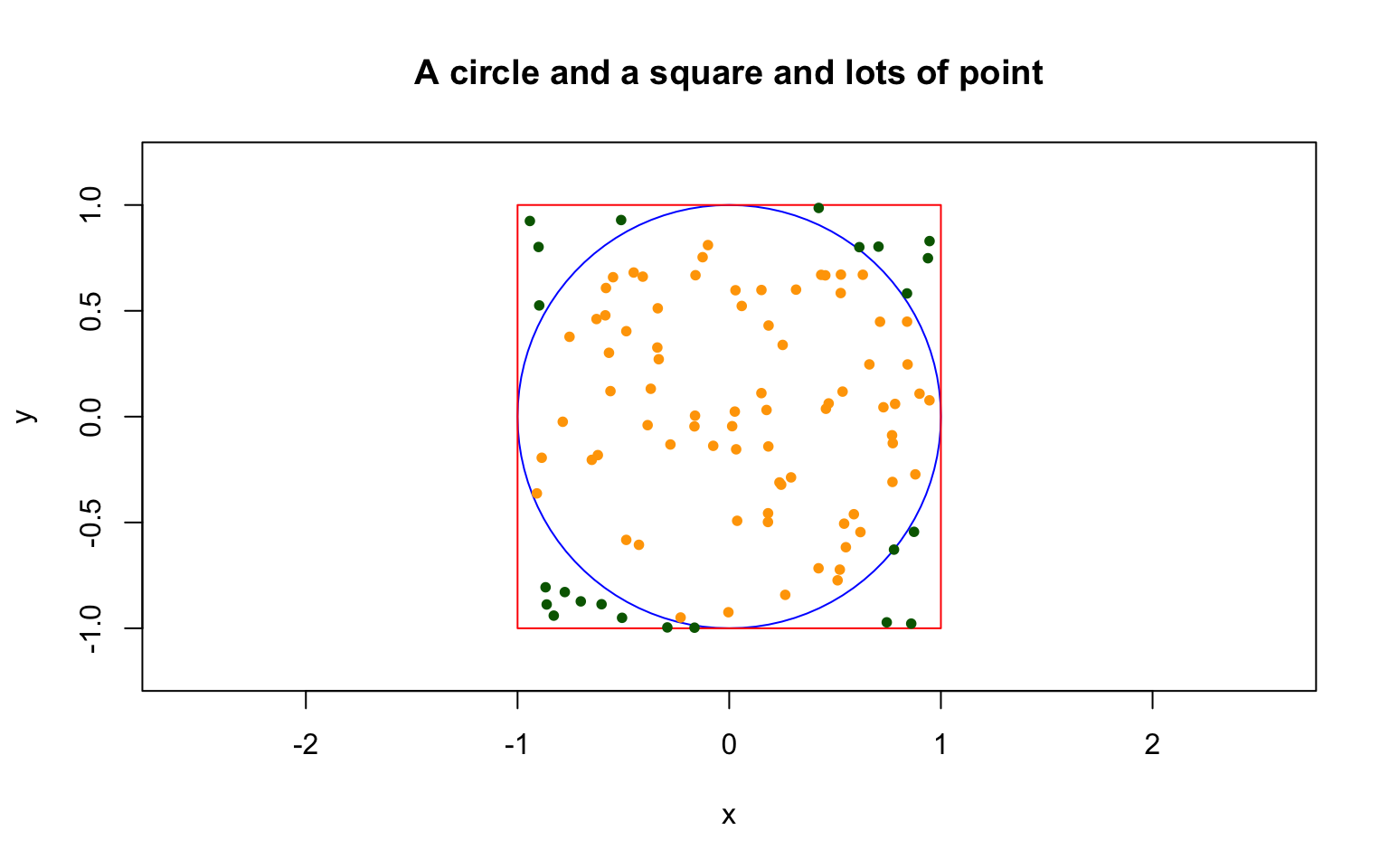
Then perfectly draw a square around our circle:

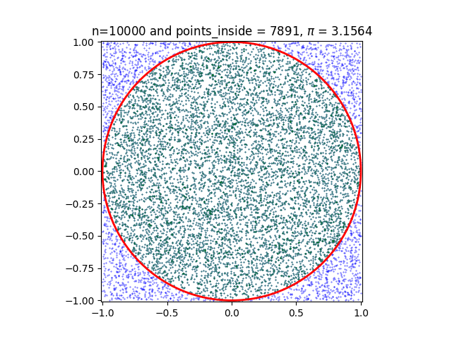
🎯 Simulate Points

Then simulate a lot of points uniformly within the square:

🧮 Compute the Proportion

From \(n=100\) points

Here we have 77 points within the circle, and so we compute

\[ \pi \approx 4 \times 0.77 = 3.08. \]

• This is clearly not a very good approximation of \(\pi\).
• We have only simulated 100 points and so we have a high variance in our estimate.

Increasing accuracy!

⬆️ To increase our accuracy we increase the number of simulations.

Let’s up our simulation count from 100 points to 100,000 points and see what approximation we get.

📈 Increasing Accuracy

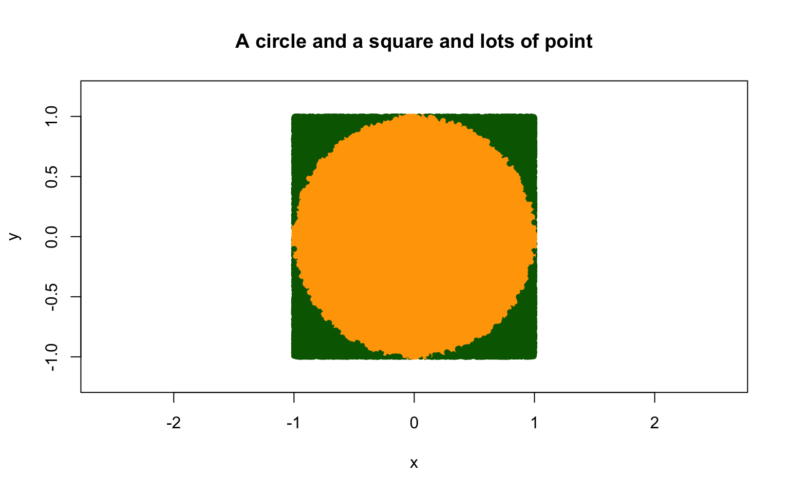
Here our approximation is 3.13816.

📊 Convergence to \(\pi\)

Let’s see how our estimate converges as we increase the number of simulated points \(n\).

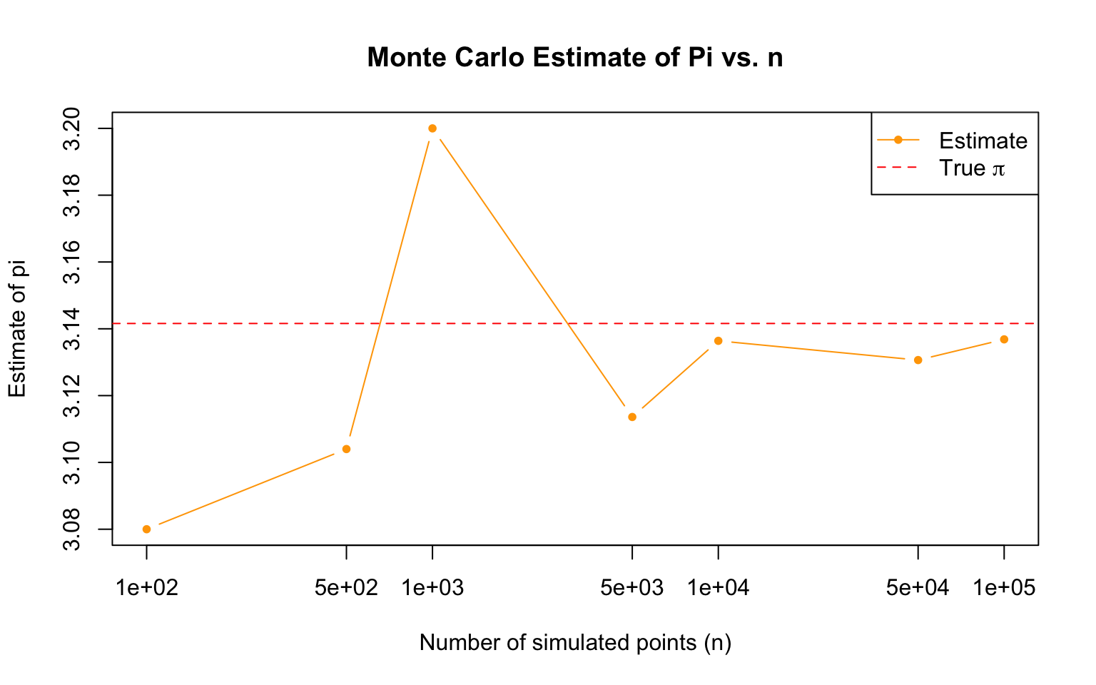
📌 As \(n\) grows, the estimate settles down around the true value \(\pi \approx 3.14159\) — the same long-run averaging behaviour we saw earlier with expectation.

Monte Carlo Methods

🎲 Monte Carlo Methods

What are Monte Carlo Methods?

Monte Carlo (MC) methods are a study of these types of problems:

• Consider a deterministic but hard to measure value (such as \(\pi\)).
• Assume we have access to controlled random sampling (e.g. runif()).
• We can approximate the deterministic value from a large number of samples.

Enrico Fermi, an early MC practitioner.

Still essential today

• Finance — pricing options and simulating portfolio risk under uncertain market conditions.
• Physics & engineering — modelling particle transport, nuclear reactions, complex systems.
• Machine learning & statistics — approximating intractable integrals in Bayesian inference.
• Operations research — estimating outcomes for scheduling, logistics, and queuing problems.

⏱️ MC Considerations — Computational Cost

Consideration 1: Time and computation effort.

Let’s compare how long it takes to simulate 100 versus 1,000,000 random values:

t1 <- Sys.time()
rands <- runif(100)
t2 <- Sys.time()
t2 - t1

Time difference of 0.001812935 secs

t1 <- Sys.time()
rands <- runif(1000000)
t2 <- Sys.time()
t2 - t1

Time difference of 0.01979899 secs

• Simulating more values takes more time, even though each individual draw is essentially instant.
• For large-scale simulations (millions or billions of trials), this added computation time can become a real bottleneck.
• There is a direct trade-off between accuracy and runtime — more samples generally means better accuracy, but longer to compute.

⏱️ MC Considerations — Error Bounds

Consideration 2: Error bounds.

Let’s compare the absolute error of our \(\pi\) estimate using \(m=100\) versus \(m=100{,}000\) samples:

# estimating pi using our previous method
m <- 100; x <- runif(m, -1, 1); y <- runif(m, -1, 1)
distances <- sqrt(x^2 + y^2)
est <- length(which(distances < 1)) * 4 / m
(error <- abs(est - pi))

[1] 0.1384073

m <- 100000; x <- runif(m, -1, 1); y <- runif(m, -1, 1)
distances <- sqrt(x^2 + y^2)
est <- length(which(distances < 1)) * 4 / m
(error <- abs(est - pi))

[1] 0.001872654

• The error shrinks as we increase the number of samples \(m\).
• However, this reduction in error is not free — it comes at the cost of extra computation time, as we saw previously.
• In general, MC error decreases at a rate of roughly \(1/\sqrt{m}\), so quadrupling the sample size only halves the error.

⚖️ Evaluating MC Methods

Considerations

These considerations are essential in evaluating MC methods.

• How quickly can we simulate trials?
• What sort of error do we have?
• How fast does the approach converge?

Ideal Situation

A method that is easy to do (fast sampling), with predictable error rates that rapidly converges to the true value.

• This usually doesn’t exist!
• Generally need to make a trade off between speed and accuracy.

Buffon’s Needle

🪡 Buffon’s Needle

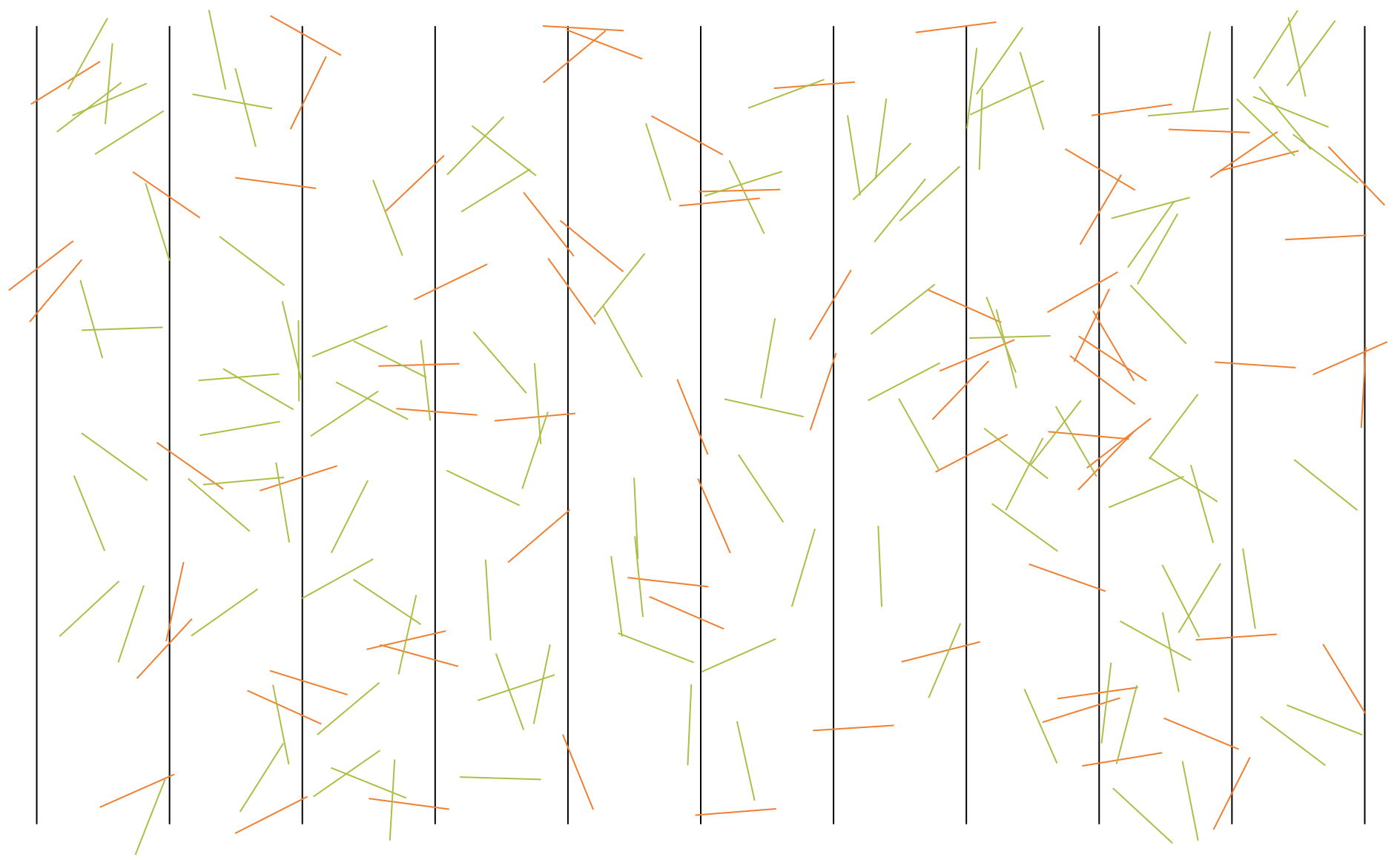
Buffon’s needle is a famous thought problem from the 1700s:

• Suppose we have a floor made out of wooden planks evenly spaced some distance d apart.
• If we drop a needle of length 1 onto the floor, what is the probability that it crosses between two planks?

Buffon’s Needle

🪡 Buffon’s Needle — Simplest Case

Interestingly, the probability \(p\) has a closed form expression which we can rearrange to estimate \(\pi\):

\[ p = \frac{2}{\pi}\times \frac{1}{d} \implies \pi = \frac{2}{p} \times \frac{1}{d}. \]

We will simulate the simplest case:

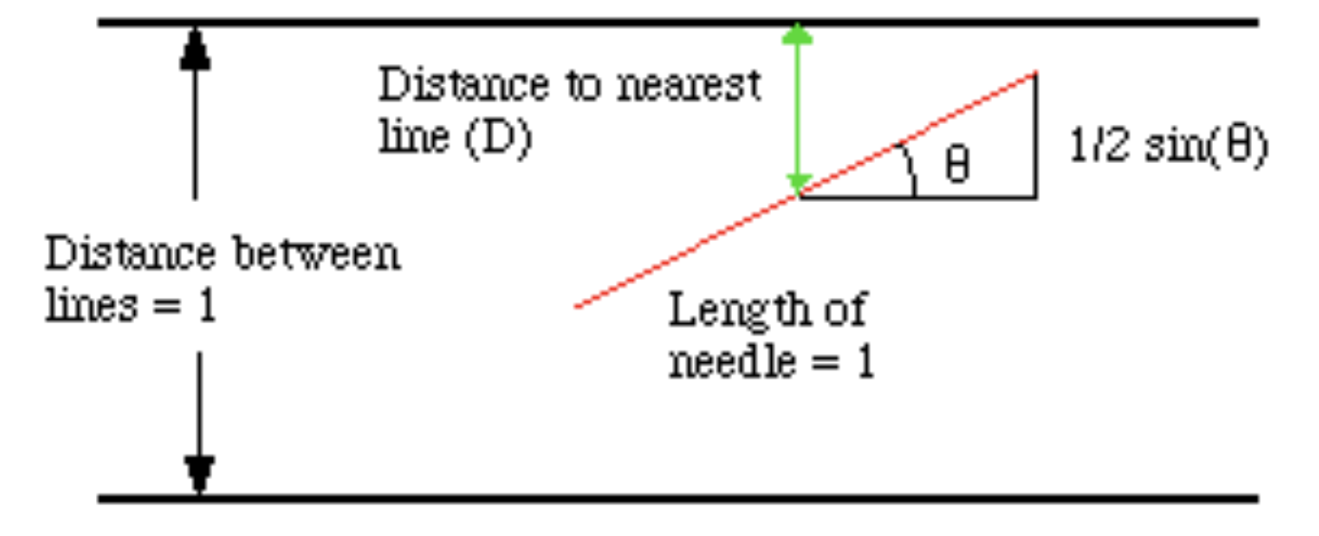
• Board distance \(d = \text{needle length} = 1\)
• Needle angle \(= \theta\)
• Distance from needle center to nearest plank \(=D\)
• Needle intersects lines when \(D > 0.5 \times \sin(\theta)\).

Buffon’s Needle Diagram

🪡 Buffon’s Needle Diagram

Buffon’s Needle Diagram

🪡 Buffon’s Needle Simulation

We conduct the following simulation:

m <- 1000

D <- runif(m, 0, 0.5) # randomly place needle centers
theta <- runif(m, 0, pi) # randomly select angles
p <- sum(D < 0.5*sin(theta))/m # number with D < 0.5*sin(θ)

• D <- runif(m, 0, 0.5) simulates the distance from the needle’s center to the nearest plank, uniform between \(0\) and \(0.5\).
• theta <- runif(m, 0, pi) simulates the angle of the needle, uniform between \(0\) and \(\pi\).
• p <- sum(D < 0.5*sin(theta))/m computes the proportion of needles that cross a plank — our estimate of \(p\).

We obtain the following estimate for \(\pi\).

(pi_est <- 2/p)

[1] 3.115265

🪡 Buffon’s Needle — Increasing Accuracy

We can increase our accuracy by increasing our simulation count.

m <- 1000000

D <- runif(m, 0, 0.5) # randomly place needle centers
theta <- runif(m, 0, pi) # randomly select angles
p <- sum(D < 0.5*sin(theta))/m # number with D < 0.5*sin(θ)

We obtain the following new estimate for \(\pi\).

(pi_est <- 2/p)

[1] 3.144239

• Increasing \(m\) from 1,000 to 1,000,000 gives us a much closer approximation to the true value of \(\pi\).
• This mirrors exactly what we saw with our circle-and-square approach earlier — more samples means lower error, at the cost of additional computation.
• Buffon’s needle is a nice illustration that MC estimation isn’t limited to one setup — many different random experiments can be engineered to approximate the same constant.

Euler’s Number

🔢 Euler’s Number

Another interesting mathematical constant is Euler’s number \(e\).

exp(1)

[1] 2.718282

We have worked with \(e\) every time we have used the exp() function, which is defined as:

\[ \exp(x) = e^x \]

i.e. raising \(e\) to the power of the input of the function.

• It is therefore the base of the natural logarithm \(\ln\).
• It also appears in a large number of the standard distribution functions (e.g. Poisson, Exponential, Normal, Gamma).

💪 Exercise — Lex Fridman Problem

05:00

Consider how we might estimate \(e\) with Monte Carlo simulation.

Lex Fridman Problem

Write and replicate a function that:

1. Selects numbers with runif() until the sum is \(>1\);
2. Determines how many selections it takes; and
3. Repeats m=10000 times to approximate \(e\).

✅ Solution — Lex Fridman Problem

above_one <- function() {
  i <- 0
  count <- 0

  while (i < 1) {
    i <- i + runif(1, 0, 1)
    count <- count + 1
  }
  return(count)
}

m <- 10000
mean(replicate(m, above_one()))

[1] 2.7186

• above_one() keeps drawing uniform random numbers and adding them to a running total i, counting how many draws it takes until that total exceeds \(1\).
• count is therefore the number of draws needed for a single trial’s running sum to pass \(1\).
• mean(replicate(m, above_one())) repeats this trial m=10000 times and averages the counts, giving our Monte Carlo estimate of \(e\).

Golden Ratio

🌀 Golden Ratio

The golden ratio \(\phi\) is another important mathematical constant, which is defined as

\[ \phi = \frac{a}{b}\quad s.t.\quad \frac{a+b}{a} = \frac{a}{b}. \]

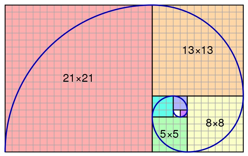
We have encountered \(\phi\) previously when working with the Fibonacci sequence.

Golden Ratio

🌀 Golden Ratio MC Estimation

We estimate the golden ratio as follows:

1. Generate pairs of numbers \(a,b\) such that \(a>b\) at random;
2. Compute \(U = (a+b)/a\) and \(L=a/b\) for each pair;
3. Compute the ratio of \(U/L\); and
4. Return the \(a,b\) values giving \(U/L\) closest to 1.

📌 This approach requires many trials.

golden <- function() {
  a <- runif(1, 0, 1)
  b <- runif(1, 0, a)
  U <- (a + b) / a
  L <- a / b
  ratio <- U / L
  return(c(ratio, a, b))
}
vals <- replicate(10000, golden())
estimates <- which.min(abs(vals[1,] - 1))
(phi <- vals[,estimates][2]/vals[,estimates][3])

[1] 1.618337

📌 Recall that the actual value is: 1.61803…

🌀 Golden Ratio Convergence

Let’s see how our estimate converges as we increase the number of trials \(m\).

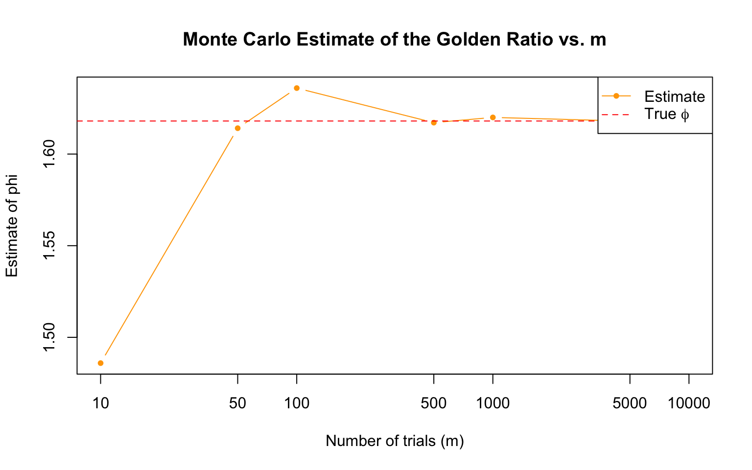
📌 As \(m\) grows, the estimate settles down around the true value \(\phi \approx 1.61803\).

Monte Carlo Integration

∫ Monte Carlo Integration

We can approximate integrals

We compute the following integral via simulation

\[ \int_0^5 x^3 dx. \]

Granted this is not a very interesting integral, but at least it is quite simple.

Idea: Express the integral as the expectation of a random variable, say \(X\sim\mathcal{U}(0,5)\) with PDF

\[ f_X(x) = \frac 15\quad \text{for}\quad 0<x<5. \]

∫ Rewrite the Integral

We can rewrite the integral as follows:

\[ \begin{aligned} \int_0^5 x^3 dx & = \int_0^5 5x^3 \times 1/5 ~dx \\ & = \int_0^5 5x^3 f_X(x)~dx \\ & = \mathbb{E}[5X^3]. \end{aligned} \]

Where \(X\sim\mathcal{U}(0,5)\). The problem reduces to:

• Simulating many \(\mathcal{U}(0,5)\) random variables;
• Cubing all simulations and multiplying them by 5;
• Taking the mean to estimate the integral.

∫ Approximate the Integral

Integrating by MC

set.seed(24)
m <- 10000
sims <- runif(m, 0, 5)
mean(5 * sims^3)

[1] 154.0979

Computing the actual value analytically we have:

\[ \int_0^5 x^3dx = \left[\frac{x^4}{4}\right]_0^5=\frac{5^4}{4} = 156.25. \]

• Here we could easily compute the integral analytically, so simulation wasn’t strictly necessary.
• This approach becomes genuinely useful when the integral is not tractable — e.g. it has no closed form, or is too high-dimensional to solve by hand.
• MC integration only requires that we can simulate from and evaluate the function — no calculus required!

The Monty Hall Problem

🚪 The Monty Hall Problem

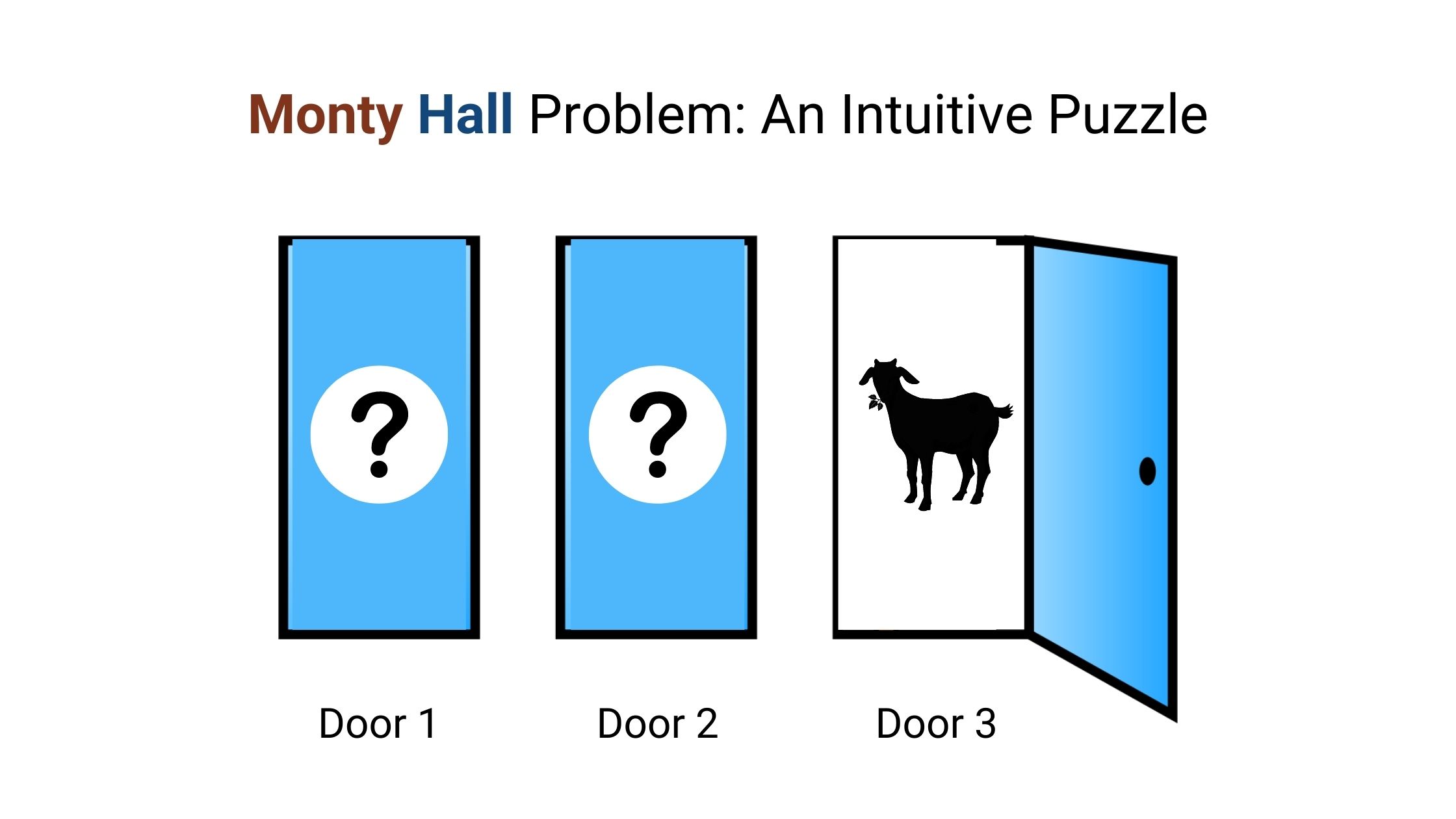
The Monty Hall problem is another famous probability puzzle with the following setup:

• You are a contestant on a game show;
• You are shown three doors: a new car is behind one door and a goat is behind each of the others;
• You select a door at random and have the chance to keep whatever is behind the door;
• After choosing a door, the show host opens one of the two remaining doors to show a goat, at which point they ask you whether you would like to change your guess.

📌 Question: Should you change your guess?

Monty Hall Problem

🚪 The Monty Hall Solution

Solution: It is always better to switch doors!

Computing the odds of winning using conditional probability we find that:

• your odds of winning if you choose to stay are \(1/3\); whilst
• your odds of winning if you choose to change are \(2/3\).

This seems counter intuitive! Surely it is just 50/50, i.e. \(1/2\) for both — there are two doors and 1 is the winner?

🚪 Monty Hall Simulation

monty_hall_game <- function(strategy) {
  prize_door <- sample(1:3, 1) # set door with car
  player_choice <- sample(1:3, 1) # set player choice
  remaining_doors <- setdiff(1:3, c(prize_door, player_choice))
  if (length(remaining_doors) == 1) { revealed_door <- remaining_doors}
  else { revealed_door <- sample(remaining_doors, 1)} # open door
  if (strategy == "stay") { # stay put
    final_choice <- player_choice
  } else { # switch doors
    options <- setdiff(1:3, c(revealed_door, player_choice))
    if (length(options) == 1) {
      final_choice <- options
    } else {
      final_choice <- sample(options, 1)
    }
  }
  win <- final_choice == prize_door; return(win)
}

• monty_hall_game() plays one round of the game for a given strategy ("stay" or "switch") and returns whether the player won.
• It randomly places the prize and the player’s initial choice, then has the host reveal a goat door from whatever remains.
• Depending on the strategy, the player’s final choice is either their original pick or the one remaining unopened door.
• We’ll break this function down line by line on the next slide.

🚪 Monty Hall Simulation Breakdown

We initially set the door with the prize, selected door and remaining door.

monty_hall_game <- function(strategy) {
  prize_door <- sample(1:3, 1)
  player_choice <- sample(1:3, 1)
  remaining_doors <- setdiff(1:3, c(prize_door, player_choice))

We then simulate the host picking a door.

  if (length(remaining_doors) == 1) {
    revealed_door <- remaining_doors
  } else {
    revealed_door <- sample(remaining_doors, 1) # open door
  }

We then decide whether to switch or stick with the current door.

  if (strategy == "stay") {
    final_choice <- player_choice
  } else {
    options <- setdiff(1:3, c(revealed_door, player_choice))
    if (length(options) == 1) {
      final_choice <- options
    } else {
      final_choice <- sample(options, 1)
  }

  win <- final_choice == prize_door

  return(win)

🚪 Testing the Claim

Let’s use our simulation to test the claim that switching is better, by playing many games under each strategy.

set.seed(24)
m <- 10000
mean(replicate(m, monty_hall_game("stay")))

[1] 0.3384

mean(replicate(m, monty_hall_game("switch")))

[1] 0.6578

• Staying wins about 1/3 of the time, and switching wins about 2/3 of the time — exactly matching our theoretical solution.
• This is a great example of using simulation to sanity-check a counter-intuitive probability result, without needing to trust the maths alone.
• The larger we make m, the closer these simulated win rates get to the true \(1/3\) and \(2/3\) probabilities.
• This same general strategy — write a function for one trial, replicate it many times, and average the results — is exactly how we approached every Monte Carlo problem in this lecture.

Summary

✅ Topics Covered

🤔 We have now looked through several examples of more complex simulation, including simulating:

• Pi
• Buffon’s Needle
• Euler’s Number
• Golden Ratio
• Integrals
• Monty Hall Problem

📌 That’s all we need for probability in PSTAT 10!

📅 Next Class

🤩 Next class we will be moving away from RStudio and will instead be focusing on:

• Databases; and
• Introduction to SQL.