PSTAT 10 Data Science Principles

Lecture 5: Algorithms

John Robin Inston

johninston@ucsb.edu

University of California, Santa Barbara

August 22, 2026

Introduction

🔁 Review: Lecture 4

👈 Last lecture we explored some automation methods such as:

Functions
Branching (if, else, else if)
Looping:
- For Loops
- While Loops
- Repeat & Break Loops
Control Flow

👀 Outline: Lecture 5

👇 This lecture we will shift our focus to problem solving, including:

Algorithmic Thinking
Branching Logic
Iterative Logic
Recursive Logic

Algorithms

📊 Data Science

What is Data Science?

Data science is a combination of subjects including:
- ➕ Math
- 📊 Statistics
- 👨‍💻 Programming
- 💻 Computer Science
- 🤖 Machine Learning

Data All Around Us

Data is the single most prolific commodity in the world with over 1 trillion GB being generated per day.
This is far too much for any human to handle, so we are required to develop automated procedures using algorithms.

🧮 What is an Algorithm?

Algorithm

An algorithm is a process / set of rules performed sequentially to solve some kind of problem.

The rules are often mathematical but can be thought of as general functions.
We have all used algorithms before, particularly in math classes whenever we learned to solve a problem in several steps: calculus and integral rules, long division, algebra etc.

🌳 Branching Algorithms

Branching Algorithm

Branching algorithms can be visualized as a case-dependent tree structure, where each branch determines which steps the algorithm applies.

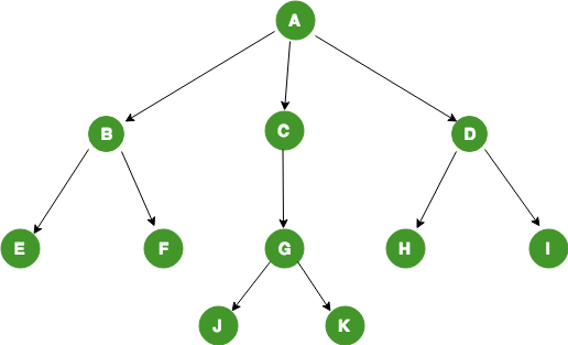
Example — Branching Algorithm

Checking the length of a character string

Here is a simple example of a branching algorithm that checks that the length of a character string is greater than 5 characters.
If the string is greater than 5 characters, the algorithm returns TRUE, otherwise it returns FALSE.

# Define the algorithm 
check_string_length <- function(string) {
  if (nchar(string) > 5) {
    return(TRUE)
  } else {
    return(FALSE)
  }
}
# Test the algorithm
check_string_length("Hello world!")

[1] TRUE

For more complicated logic, we can use nested branching to check multiple conditions in a single algorithm.

🪆 Nested Branching Statements

Branching statements can be nested inside one another — an if / else if / else block can contain another complete branching block.

This is useful when a decision depends on more than one condition, checked one at a time.
The general structure looks like:

if (logical1) {
  if (logical2) {
    ACTION A
  } else {
    ACTION B
  }
} else {
  ACTION C
}

Syntax Tips

Indent each nested level further than the block containing it — this makes the structure easy to read at a glance.
Every opening brace { needs a matching closing brace } — close the inner block before the outer one.
RStudio auto-indents and highlights matching braces for you — use this to check your work!

🪆 Example — Nested Branching

Suppose we want to classify a temperature, but “hot” vs “cool” means something different depending on whether it’s a weekday or a weekend:

classify_day <- function(temp, weekday) {
  if (weekday) {
    if (temp > 75) {
      return("Hot workday")
    } else {
      return("Cool workday")
    }
  } else {
    if (temp > 85) {
      return("Hot weekend")
    } else {
      return("Cool weekend")
    }
  }
}
classify_day(80, TRUE)

[1] "Hot workday"

📌 Notice the outer branch picks weekday vs weekend, and the inner branch then checks the temperature within it — exactly the pattern you’ll need for the next exercise!

💪 Exercise — Nested Branching Practice

04:00

Write a function check_number that takes a single numeric input x and uses nested branching as follows:

First check whether x is positive or non-positive (zero or negative).
If x is positive, nest a second branch that checks whether x is even or odd, returning "positive even" or "positive odd".
If x is non-positive, nest a second branch that checks whether x is zero or negative, returning "zero" or "negative".

Hint: the modulo operator %% is helpful for checking even / odd — recall x %% 2 == 0 when x is even.

✅ Solution — Nested Branching Practice

check_number <- function(x) {
  if (x > 0) {
    if (x %% 2 == 0) {
      return("positive even")
    } else {
      return("positive odd")
    }
  } else {
    if (x == 0) {
      return("zero")
    } else {
      return("negative")
    }
  }
}

check_number(4)
check_number(-7)
check_number(0)

[1] "positive even"

[1] "negative"

[1] "zero"

📌 Notice the outer branch (positive vs. non-positive) is fully resolved — including both its nested branches closed off with } — before the else for the outer branch even appears.

💪 Exercise — Branching Algorithms (Word Search)

05:00

Consider the following lang_matrix:

lang_matrix <- rbind(
  c("hello", "goodbye", "friend"),
  c("hola", "adios", "amigo"),
  c("bonjour", "au revoir", "ami")
)
print(lang_matrix)

     [,1]      [,2]        [,3]    
[1,] "hello"   "goodbye"   "friend"
[2,] "hola"    "adios"     "amigo" 
[3,] "bonjour" "au revoir" "ami"

Define this matrix.
Write a function word_search with two character string inputs: language (english, spanish or french) and type (greeting, farewell or friend).
The function should return the cell corresponding to the language and greeting term.

For example:

word_search("french", "greeting")

[1] "bonjour"

✅ Solution — Branching Algorithms (Word Search)

An inefficient first attempt:

word_search <- function(a, b) {
  if (a == "english" | a == "e") {
    if (b == "greeting") {return(lang_matrix[1, 1])}
    else if (b == "farewell") {return(lang_matrix[1, 2])}
  }
  else if (a == "spanish" | a == "s") {
    if (b == "greeting") {return(lang_matrix[2, 1])}
    else if (b == "farewell") {return(lang_matrix[2, 2])}
  }
  else if (a == "french" | a == "f") {
    if (b == "greeting") {return(lang_matrix[3, 1])}
    else if (b == "farewell") {return(lang_matrix[3, 2])}
  }
  else{ print("ERROR: word not found")}
}

✅ Solution — A Better Approach

To demonstrate that there are various ways to accomplish the same task we introduce the function %in%, which tests whether a value is in a vector.

3 %in% c(1, 2, 3, 4, 5) # TRUE

[1] TRUE

6 %in% c(1, 2, 3, 4, 5) # FALSE

[1] FALSE

# more efficient solution using %in%
word_search <- function(language, type) {
  # Name the matrix indices
  dimnames(lang_matrix) <- list(c("english", "spanish", "french"),
                                c("greeting", "farewell", "friend"))
  # Use named indices
  if(
    language %in% c("english", "spanish", "french") &
    type %in% c("greeting", "farewell")
  ) {
    return(lang_matrix[language, type])
  } else {
    print("Error: Word not found!")
  }
}

🔁 Iterative Algorithms

Inefficiency of Branching Algorithms

Branching algorithms are often excellent choices but they come with some limitations:

Larger numbers of branches are time consuming to program manually.
Inefficient for traversing objects of indeterminate length.

# Example of inefficient branching algorithm
bad_in_vector <- function(v) {
  if (v[1] == 1) {print("1 is in the vector")}
  else if (v[2] == 1) {print("1 is in the vector")}
  else if (v[3] == 1) {print("1 is in the vector")}
  else if (v[4] == 1) {print("1 is in the vector")}
  else if (v[5] == 1) {print("1 is in the vector")}
  else if (v[6] == 1) {print("1 is in the vector")}
  else if (v[7] == 1) {print("1 is in the vector")}
  else {print("1 is not in the vector")}
}

What are Iterative Algorithms?

Iterative Algorithm

An iterative algorithm is a process that repeats a set of instructions until a specific condition is met.

🔁 Example — Iterative Algorithm

Suppose we want to count how many negative numbers appear in a vector. An iterative algorithm repeats the same check for every element:

count_negatives <- function(v) {
  count <- 0
  for (i in 1:length(v)) {
    if (v[i] < 0) {
      count <- count + 1
    }
  }
  return(count)
}
count_negatives(c(3, -2, -7, 5, -1))

[1] 3

📌 Notice the pattern: loop over every index, check a condition, then update something — this is exactly the structure you’ll use in the next exercise!

💪 Exercise — Iterative Algorithms

03:00

Write a function alter_entry that:

Takes a vector (of any data type) as input, and
Returns the same vector, but replacing every instance of the number 7 in the vector with 0.

Below are some examples of the function output:

alter_entry(c(7,2,3,7,1))
alter_entry(c(10, 7, 3, 7, 8))

[1] 0 2 3 0 1

[1] 10  0  3  0  8

✅ Solution — Iterative Algorithms

First we construct the surrounding function.
Then we define the for loop iterating over the indices of the input vector.
Each iteration checks whether the value at the current index is equal to 7. If it is, we replace it with 0.

# define alter_entry function
alter_entry <- function(v) {
  for(i in 1:length(v)) {
    if(v[i] == 7){
      v[i] <- 0
    }
  }
  return(v)
}

alter_entry(c(7,2,3,7,1))
alter_entry(c(10, 7, 3, 7, 8))

[1] 0 2 3 0 1

[1] 10  0  3  0  8

Remember you should still always try to avoid looping when possible.
- Lets see if we can improve the efficiency of our previous function by introducing the which() function.

🔎 The `which()` Function

A very helpful function!

Often we would like to return the indices of the elements of a vector that satisfy a certain condition.
- For this we can use the which() function.
- The which() function takes a logical vector as input and returns the indices of the TRUE values.
- It can be helpful for avoiding iterative logical queries!
An alternative solution to our previous example using the which() function could be:

alter_entry <- function(v) {
  v[which(v == 7)] <- 0
  return(v)
}

📌 Which function is more efficient?

🌀 Fibonacci Sequence

In preparation for the next exercise we briefly introduce the Fibonacci sequence.

The Fibonacci sequence is a mathematical pattern occurring commonly in nature. It appears in the golden ratio, which is found in petals, seashells, and galaxy spirals.

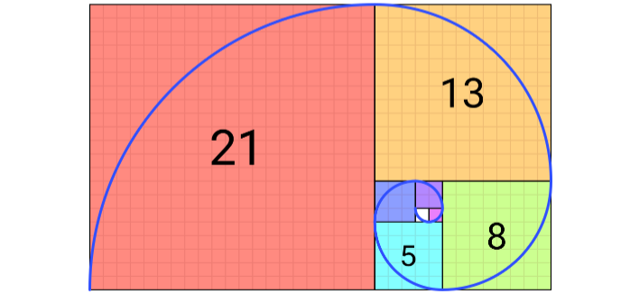
The sequence itself is constructed by starting with the initial values \(0\) and \(1\), and every subsequent value is the sum of the previous two, i.e.

\[ x_n = x_{n-1} + x_{n-2}; \quad x_1 = 0, \quad x_2 = 1. \]

💪 Exercise — Fibonacci Sequence

05:00

Write an iterative function fib_n that returns the \(n\)-th term of the Fibonacci sequence:

The function should take one numerical scalar input n.
The function should return a numeric value representing the \(n\)-th term of the Fibonacci sequence.
Ignore exception cases and do not worry about robustness — assume the input will always be a positive integer.

fib_n(10)
fib_n(25)

[1] 34

[1] 46368

✅ Solution — Fibonacci Sequence

We start once again by defining the function and its input.
Next we define the base cases for the first two terms of the Fibonacci sequence.
Finally we define a for loop that iteratively calculates the Fibonacci sequence up to the \(n\)-th term.

# define fib_n function
fib_n <- function(n){
  if(n == 1) {
    return(0)
  } else if (n==2) {
    return(1)
  } else {
    temp <- c(0,1)
    for(i in 3:n){
      temp[i] <- temp[i-1] + temp[i-2]
    }
    return(temp[n])
  }
}

fib_n(10)
fib_n(25)

[1] 34

[1] 46368

🧩 Combining Everything

Notice that in our previous example we were required to use both branching and iteration. It is common for algorithms to require the use of several tools.

To understand and eventually design algorithms it is important to know how the individual pieces / steps work and what they are doing.

Certain tricks come up more often than others, such as:

Iterating through vector indices (enumeration);
Storing and updating temporary or intermediate values; and
Utilizing data structure and specific behavior.

Let’s see if we can combine these tools to solve a problem in the next exercise!

💪 Exercise — Last Negative

05:00

Combine some of the tools we have been studying by defining a function called last_negative that:

Takes a numeric vector v.
Returns the last (index-wise) negative value in v and its index (in a 2-element vector).
If v does not have any negative values, returns the character string "No negative values".

Below are some examples of the function output:

last_negative(c(-1,2,6,-2,8,-9))
last_negative(c(5,2,1,4,5,6,9))

[1] -9  6

[1] "No negative values"

✅ Solution — Last Negative

We start by defining the function and its input.
Next we define a temporary variable temp to store the last negative value and its index, or a message if no negative values are found.
Finally we define a for loop that iterates through the vector, checking for negative values and updating temp accordingly.

last_negative <- function(v) {

  temp <- "No negative values" # storing tempory vector

  for(i in 1:length(v)){
    if(v[i] < 0) {
      temp <- c(v[i], i)
    }
  }
  return(temp)
}

last_negative(c(-1,2,6,-2,8,-9))
last_negative(c(5,2,1,4,5,6,9))

[1] -9  6

[1] "No negative values"

Nested Loops

🪆 Nested Loops

Sometimes we may wish to run loops inside other loops (e.g. iterating over first the rows and then the columns of a matrix), and to do so we use nested loops.

Example Nested For Loop

for(LOGICAL1, often index-based) {
  DO OPERATION1

  for(LOGICAL2, often index-based){
    DO OPERATION2
  }
}

Nested loops are useful but slow!
Good practice is to only use them when necessary, prioritising vectorized solutions.

💪 Exercise — Two Sum

05:00

Write a function called two_sum that:

Takes an input vector v and a numerical scalar target, and
Returns the indices of the two entries of v that add up to the target.

Assume that:

Two indices cannot be equal (i.e. target will not be twice any value in v);
If no values summing to target are found, return NULL; and
Only one such pair of elements in v sum to the target.

two_sum(c(5,6,0,1,4),11)

[1] 1 2

✅ Solution — Two Sum

# define two_sum function
two_sum <- function(v, target) {
  n <- length(v)
  for (i in 1:(n - 1)) {
    for (j in (i + 1):n) {
      if(v[i] + v[j] == target) {
        return(c(i, j))
      }
    }
  }
return(NULL)
}

📌 See whether you can design a more efficient function using vectors!

Searching & Sorting

🔍 Searching & Sorting

Famous Problems

Two very famous problems in computer science are:

How to search data structures for specific values; and
How to sort unsorted numerical vectors.

R has built in functions to handle both of these problems (i.e. sort() and %in%) but to understand the challenges of these problems we take a look at two specific solutions:

Bubble sorting
(Iterative) binary searching

🫧 Bubble Sort

In 2007, former Google CEO Eric Schmidt asked then presidential candidate Barack Obama during an interview about the best way to sort one million integers.

Obama paused for a moment and replied “I think the bubble sort would be the wrong way to go.”

🫧 The Bubble Sort Algorithm

Main Idea

Assume our input is a (potentially long) vector v of unsorted values.
The idea is that we let the “lighter” values “sink” to the bottom.
Apply the following algorithm:
- Iterate through the entire vector.
- For every pair of indices j and j+1, if v[j] > v[j+1] swap the values at those indices.
- Stop iterating when the vector is fully sorted.
- The desired output is a vector containing the sorted values of v.

Example — Defining Bubble Sort

Implementation

bubble_sort <- function(v) {
  n <- length(v)
  for (i in 1:(n - 1)) { # iterate through n-1 loops
    is_swapped <- FALSE
      for (j in 1:(n - i)) { # swap values at specific indices
        if (v[j] > v[j + 1]) {
          temp <- v[j]
          v[j] <- v[j + 1]
          v[j + 1] <- temp
          is_swapped <- TRUE
        }
      }
    if (!is_swapped) { # break out of loop if fully sorted
      break
    }
  }
return(v)
}

Testing the Algorithm

As an example of our algorithm in action let’s define a vector of 30 numbers in a random order:

bubble_sort_test <- sample(1:100, 30, replace = FALSE)
bubble_sort_test

 [1]   3  14  10  25  30  47  79  32  67  29  28  92 100  22   4  16  94  37  46
[20]  35  50  52  12  13  90  95  55  53   5  59

We apply the bubble sort algorithm:

bubble_sort(bubble_sort_test)

 [1]   3   4   5  10  12  13  14  16  22  25  28  29  30  32  35  37  46  47  50
[20]  52  53  55  59  67  79  90  92  94  95 100

🎯 Binary Search

Idea behind Binary Search

Assume that I have picked a number between 1 and 1024 and tell you to guess which number I have chosen.
- You can only use higher or lower as clues.
- You have to guess the correct number in 11 or fewer attempts.
Can you design an algorithm that always guesses correctly?

Binary Search Structure

The general structure of the binary search algorithm is as follows:

Begin with a sorted vector v and a target value target.
If the midpoint of v equals the target, end.
- If the midpoint is greater (less) than target, repeat the previous step with the midpoint of the upper (lower) half of the vector.
Repeat until target is found.

🎯 Binary Search Algorithm

Implementation

# define binary search algorithm
binary_search <- function(v, target) {
  left <- 1
  right <- length(v)
  while (left <= right) {
    mid <- floor((left + right) / 2) # check the vector midpoint
    if (v[mid] == target) {
      return(mid)
    } else if (v[mid] < target) { # check lower
      left <- mid + 1
    } else {
      right <- mid - 1
    }
  }
  return(NULL)
}

Binary Search Example

# define a sorted vector
test_vector <- c(1, 3, 5, 7, 9, 11, 13, 15, 17, 19)
binary_search(test_vector, 7) # returns 4

[1] 4

🔄 Recursion

Recursion is another common algorithmic pattern.

It is the act of defining a problem in terms of simpler versions of itself.
Recursion consists of a base case and a recursive step.

# recursion general form
recursion <- function(INPUTS) {
  if (TERMINATION CONDITION) { # base case
    END RECURSIVE FUNCTION
  } else {
    new_inputs <- DO SOMETHING # recursive step
    recursion(new_inputs)
  }
}

🌀 Example — Recursive Fibonacci

Recall that we previously wrote an iterative Fibonacci algorithm.

Iterative approaches are effective, and our previous function worked perfectly.
However, iterative setups can be complicated to implement.
Furthermore, the main drawback of iteration is typically computational cost and time — it is often not very efficient!

Let’s try using recursion to create a new version of the fib_n function.

We have the same setup: take an input \(n\) and return the \(n\)-th term of the Fibonacci sequence.
This time, construct the function using recursion.

🌀 Recursive Fibonacci — Implementation

# recursive fibonacci function
fib_recur <- function(n) {
  if (n <= 2) { # base case
    return(n-1)
  }
  return(fib_recur(n - 1) + fib_recur(n - 2)) # recursive step
}
# example output
fib_recur(25)

[1] 46368

📌 The recursive Fibonacci function works exactly the same, however the implementation is much faster. The drawback is that the logic behind the implementation is less intuitive.

Summary

✅ Topics Covered

🤔 Today we began exploring problem solving:

Algorithmic Thinking
Branching Logic
Iterative Logic
Recursive Logic

📅 Next Class

🤩 Next class we look at:

Storing data
Factor data

PSTAT 10 Data Science Principles

Introduction

🔁 Review: Lecture 4

👀 Outline: Lecture 5

Algorithms

📊 Data Science

What is Data Science?

Data All Around Us

🧮 What is an Algorithm?

🌳 Branching Algorithms

Example — Branching Algorithm

Checking the length of a character string

🪆 Nested Branching Statements

Syntax Tips

🪆 Example — Nested Branching

💪 Exercise — Nested Branching Practice

✅ Solution — Nested Branching Practice

💪 Exercise — Branching Algorithms (Word Search)

✅ Solution — Branching Algorithms (Word Search)

✅ Solution — A Better Approach

🔁 Iterative Algorithms

Inefficiency of Branching Algorithms

What are Iterative Algorithms?

🔁 Example — Iterative Algorithm

💪 Exercise — Iterative Algorithms

✅ Solution — Iterative Algorithms

🔎 The which() Function

A very helpful function!

🌀 Fibonacci Sequence

💪 Exercise — Fibonacci Sequence

✅ Solution — Fibonacci Sequence

🧩 Combining Everything

💪 Exercise — Last Negative

✅ Solution — Last Negative

Nested Loops

🪆 Nested Loops

💪 Exercise — Two Sum

✅ Solution — Two Sum

Searching & Sorting

🔍 Searching & Sorting

Famous Problems

🫧 Bubble Sort

🫧 The Bubble Sort Algorithm

Main Idea

Example — Defining Bubble Sort

Implementation

Testing the Algorithm

🎯 Binary Search

Idea behind Binary Search

Binary Search Structure

🎯 Binary Search Algorithm

Implementation

Binary Search Example

🔄 Recursion

🌀 Example — Recursive Fibonacci

🌀 Recursive Fibonacci — Implementation

Summary

✅ Topics Covered

📅 Next Class

🔎 The `which()` Function