PSTAT 10 Data Science Principles

Lecture 4: Functions, Branching and Loops

John Robin Inston

johninston@ucsb.edu

University of California, Santa Barbara

August 6, 2026

Introduction

🔁 Review: Lecture 3

👈 Last lecture we started exploring higher-dimensional data structures such as:

Vectors \((1 \times n)\)
Matrices \((n \times p)\)
Arrays \((n_1 \times n_2 \times ... \times n_k)\)
Lists (ordered items)
Accessing data; creating data structures

👀 Outline: Lecture 4

👇 This lecture we look into automating repetitive tasks using:

Functions
Branching (if, else, else if)
Loops (for, while, repeat)
Control Flow

Functions

🧩 What is a Function?

In programming, a function is a self-contained, reusable block of code designed to perform a specific task.

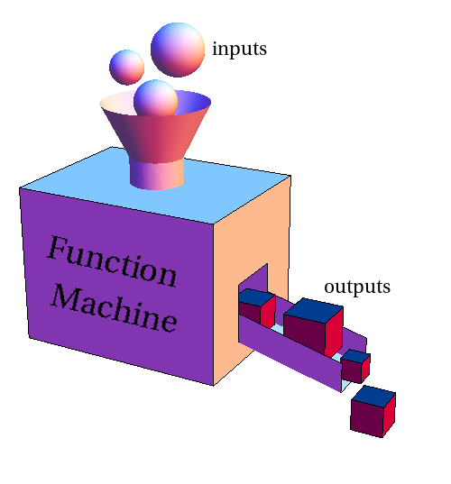
Nykamp DQ, “The function machine.” From Math Insight.

A function can take zero or more inputs and returns at least one outputs.
Writing a function lets us reuse the same logic without retyping it — a core idea in programming.

🧰 Functions in R

We have implicitly and explicitly used dozens of functions already:

Constructing Objects

c(), matrix()
array(), list()

Math & Summaries

exp(), log(), sqrt()
mean(), median(), sum()

We’ve also used functions that interact with our environment rather than our data, such as getwd() and setwd().

Some functions did not require inputs; some did not appear to produce outputs.
- In reality, all functions output something, even if it is just a setting change or manipulating objects.

🏗️ Function Anatomy

We define a function in R using the following syntax:

abstract <- function(in_1, in_2, ... , in_k) {  # input arguments

  FUNCTION MACHINE  # core of the operation

  return(outputs)  # appropriate output
}

R functions can take any number of inputs.
R functions can only return at most one output (sort of):
- We can get around this using data structures such as lists or using packages.

Example — Matrix Deconstruct Function

We wish to define a function that takes a matrix as an input and returns the first and last rows.

matrix_deconstruct <- function(x){ # input x
  # function machine
  row_dim <- dim(x)[1] # number of rows
  firstrow <- x[1,] # select first row
  lastrow <- x[row_dim, ] # select last row
  return(list(firstrow, lastrow)) # output row list
}

📌 Notice that the function we define is listed in the environment pane, just like any other object.

Example — Testing Functions

To test our function we define a \(4\times 3\) matrix and apply our function to obtain:

test_matrix <- matrix(1:12, nrow = 4, ncol = 3)
matrix_deconstruct(test_matrix)

[[1]]
[1] 1 5 9

[[2]]
[1]  4  8 12

The output is a list of two elements — the first and last rows - but one object.

We can access each element individually using double-bracket indexing:

matrix_deconstruct(test_matrix)[[1]]
matrix_deconstruct(test_matrix)[[2]]

[1] 1 5 9

[1]  4  8 12

Let’s stress-test with an edge case: a single-row matrix.

# a single-row matrix
one_row <- matrix(1:5, nrow = 1)
matrix_deconstruct(one_row)

[[1]]
[1] 1 2 3 4 5

[[2]]
[1] 1 2 3 4 5

📌 With a single-row matrix, the first and last row are the same!

💪 Exercise — Defining Functions

02:00

Take 2 minutes to attempt to define your own function.

We wish to write a function called inc_nth_root which does the following:

Takes two inputs (labels are arbitrary but let’s use v and n).
Increments v by 1 (i.e. adds 1 to v).
Computes the \(n\)th root of v (i.e. v raised to the power of \(1/n\)).
Returns the resulting value.

✅ Solution — Defining Functions

First Solution

The first solution we write is very explicitly clear but slightly inefficient:

inc_nth_root <- function(v,n){
  v <- v+1
  v <- v^(1/n)
  return(v)
}

Second Solution

The second is more efficient and returns an equivalent result:

inc_nth_root2 <- function(v,n){
  output <- (v+1)^(1/n)
  return(output)
}

✅ Solution — Testing Functions

We test our solution with the following unit tests:

c(inc_nth_root(63,3), inc_nth_root2(63,3))
c(inc_nth_root(3,2), inc_nth_root2(3,2))

[1] 4 4

[1] 2 2

Let’s consider inputs we might not have accounted for:

inc_nth_root("seal", "otter"); inc_nth_root(24,0)

Error in v + 1: non-numeric argument to binary operator

[1] Inf

📌 Always think about how people might “break” your code!

🎛️ Omitted Arguments

When defining functions we often have cases where we typically only use a handful of the arguments since the others have default inputs.

To define such a function we can specify default values of our inputs which the function will assume to be used unless the user specifies otherwise.

Improving inc_nth_root

Currently if we omit our inputs we get an error message:

inc_nth_root()

Error in inc_nth_root(): argument "v" is missing, with no default

We can define default values for our inputs to avoid this problem:

inc_nth_root <- function(v = 0, n = 2){
  v <- v+1
  v <- v^(1/n)
  return(v)
}

We have specified that if no input is provided, the function will assume v = 0 and n = 2.

inc_nth_root() # <- uses default values

[1] 1

Branching

🔀 Branching

To protect our function against other problems (such as incorrect data types) we introduce the concept of branching.

R allows branching blocks using if, else and else if statements which each do the following:

if — takes a logical input and if the input is satisfied executes the branched code.
else if — follows an if statement as a catch all, applying a second logical test when the preceding condition is not satisfied.
else — the final part of a branching block: if none of the previous branches were triggered this code is executed.

Below is a full branching block (an if/else block) using all three:

if (logical1) { # condition on 1st logic statement
  PERFORM ACTION 1 # action if logical1 is true
} else if (logical2) { # condition on 2nd logic statement
  PERFORM ACTION 2 # action if logical2 is true
} else { # only runs if previous logicals are FALSE
  PERFORM ACTION 3
}

Example — Branching

Suppose we wish to design a function that returns certain character strings describing whether the length of our vector x is below, between or above certain values.

length_test <- function(x = 0){
  if(length(x) < 10){
    print("Vector has length less than 10!")
  } else if (length(x) >= 10 & length(x) <= 20){
    print("Vector has length between 10 and 20!")
  } else {
    print("Vector has length greater than 20!")
  }
}

Notice we defined a default input value of 0 to avoid error messages!

Let’s test our function using a collection of vectors:

length_test(rep(1,15))

[1] "Vector has length between 10 and 20!"

length_test(c("dog", "cat", "monkey", "horse"))

[1] "Vector has length less than 10!"

length_test(1:100)

[1] "Vector has length greater than 20!"

🛠️ Robustifying `inc_nth_root`

Returning to our inc_nth_root function we wish to make it robust to the following problems:

Incorrect input datatypes returns an error message.
Using 0 as the \(n\) input returns Inf.
Providing a vector input returns a vector.
Omitting the \(n\) input returns an error message.

We can now fix these issues by using branching blocks.

inc_nth_root <- function(v = 0, n = 2) {  # set defaults

  if (is.numeric(v) == FALSE | length(v) != 1) {
    return("Vector v is not a numeric scalar!")
  }
  else if (n == 0) {
    return("Cannot divide by zero!")
  }
  else {
    v <- v+1
    v <- v^(1/n)
    return(v)
  }
}

📌 Notice is.numeric(v) == FALSE | length(v) != 1 is a reusable check — if we needed it in several functions, we could write it once as its own function and nest it inside each one.

🪆 Nesting Functions

Functions can call other functions inside their body — this is known as nesting functions.

Breaking a task into smaller functions makes each piece easier to write, test, and reuse.
A common use case is factoring out repeated logic — like the input check above — into its own function.

helper <- function(x) {
  CHECK OR TRANSFORM x
}

main_function <- function(x) {
  result <- helper(x)  # nested call
  return(result)
}

Example — Nesting Functions

Suppose several of our functions need to check whether an input is a valid numeric scalar. Rather than repeating the check each time, we write it once:

numeric_scalar <- function(x) {
  if (!is.numeric(x) | length(x) != 1) {
    return(FALSE)
  } else {
    return(TRUE)
  }
}

We can now nest numeric_scalar() inside inc_nth_root instead of repeating its logic:

inc_nth_root3 <- function(v = 0, n = 2) {
  if (!numeric_scalar(v)) {
    return("Vector v is not a numeric scalar!")
  } else if (n == 0) {
    return("Cannot divide by zero!")
  } else {
    v <- v + 1
    v <- v^(1/n)
    return(v)
  }
}

numeric_scalar("seal")
inc_nth_root3("seal", 2)

[1] FALSE

[1] "Vector v is not a numeric scalar!"

📌 The same numeric_scalar() helper could now validate inputs in any other function.

Testing the Robust `inc_nth_root`

Let’s see if our correction has been successful: 🥳

inc_nth_root("seal","otter")
inc_nth_root(2, 0)

[1] "Vector v is not a numeric scalar!"

[1] "Cannot divide by zero!"

inc_nth_root()
inc_nth_root(63, 3)

[1] 1

[1] 4

💪 Exercise — Defining Robust Functions

05:00

Try to define a function named is_divisible that takes two integer inputs p and q that behaves as follows:

If either p or q are not numeric then print “Error: invalid input!”
If p divides q then print “p divides q!”
If p does not divide q then print “p does not divide q!”

Hint: The modulo operator %% helps determine when p divides q:

4 %% 2 # <- 0 when divides
4 %% 3 # <- non-zero otherwise

[1] 0

[1] 1

✅ Solution — Defining Robust Functions

We can define the function using branching blocks as follows:

is_divisible <- function(p, q) {

  if (!is.numeric(p) | !is.numeric(q)) {
    print("ERROR: invalid input")

  } else if (q %% p == 0) {
    print("p divides q")

  } else {
    print("p does not divide q")
  }

}

✅ Solution — Testing Robust Functions

As a test we see that:

is_divisible(4,20)

[1] "p divides q"

is_divisible(9,100)

[1] "p does not divide q"

is_divisible("cat", 40)

[1] "ERROR: invalid input"

Loops

🔁 Iteration

One of the primary advantages of programming is the ability to iterate actions rather than repeating them manually.

Loops

In programming, iterative structures are called loops, and R has three types of looping structure:

for loops — repeat a procedure over a specified number of iterations.
- Typical use: applying the same operation to each element of a vector or each column of a data set.
while loops — repeat a procedure while a certain condition is satisfied and stop as soon as it isn’t.
- Typical use: running a simulation or optimization until it converges, when you don’t know in advance how many steps it will take.
repeat loops — the reversed while loop, repeating a procedure while a certain condition is not satisfied and stopping as soon as it is.
- Typical use: retrying an action — like drawing a random sample — until it meets some requirement.

For Loops

The most common looping structure in R is the for loop, which has the following general syntax:

for(COUNTER in RANGE){
  ACTIONS
}

We typically choose variables i, j, k for the counter and specify the range with some vector.
The actions can be dependent on the index i or not, depending on the functionality of the loop.

Example — For Loop

We wish to construct a for loop that:

iterates over the column names of the inbuilt iris data set; and
prints the number of characters in the column name.

for(i in 1:dim(iris)[2]){
  column_name <- names(iris)[i]
  char_count <- nchar(column_name)
  print(paste0(column_name, ": ", char_count))
}

[1] "Sepal.Length: 12"
[1] "Sepal.Width: 11"
[1] "Petal.Length: 12"
[1] "Petal.Width: 11"
[1] "Species: 7"

While Loops

Another helpful looping structure in R is the while loop, which has the following general syntax:

while (!TERMINATION) { # termination condition
  ACTIONS
}

While loops continue to iterate until some termination condition is TRUE.
Define the termination condition carefully as you risk having your loop run indefinitely.
While loops are useful when we don’t know exactly when they end, or when we are interested in the value of the loop index.

Example — While Loop

# Problematic while loop
i <- 0 # initialize starting condition
while(i < 3) {
  print(2 * i)
}

This loop never updates i, so the termination condition is never met — it will run forever.

# Corrected while loop
i <- 0
while(i < 3) {
  print(2*i)
  i <- i + 1
}

[1] 0
[1] 2
[1] 4

🔂 Repeat & Break

The final looping structure we consider is the repeat loop, which has the following general syntax:

repeat{
  ACTIONS
  if(CONDITION) {
    break
  }
}

Repeat & Break Example

The repeat and break loop is a reversed while structure which performs an action until the condition is met.
We don’t often use this type of loop, but still be cautious as it carries the same risks as while loops.

i <- 0
repeat {
  i <- i + 1
  if (i == 3) break
}
i

[1] 3

🚦 Control Flow

Everything we have seen so far is a type of control flow:

Sequencing (first A, then B, then C, …)
Branching (if A → ACTION, else if B → ACTION, …)
Iteration (do A1, do A2, …, STOP)

Other types of control flow include:

Non-determinacy (do A or B or C or … at random)
Concurrency (do A and B and C simultaneously)
Recursion

🧭 Thinking About Control Flow

Whenever you write or read a block of branching or looping code, it helps to explicitly ask yourself:

What is the order of execution? Code runs top-to-bottom unless a branch or loop redirects it.
Are the conditions in a branching block mutually exclusive? Could more than one — or none — ever be true?
Could a loop run zero times, once, or forever? Have you checked all three?

Trace through your code by hand with a concrete, simple input before trusting it on real data.
Ask what happens at the boundary — the first iteration, the last iteration, an empty input.

🧹 Good Practices

Keep conditions simple and readable — break complex logic into named intermediate variables or helper functions.
Avoid deeply nested if/for blocks where possible; nesting makes code harder to read, debug, and test.
Always double-check a loop’s termination condition before running it — an infinite loop can crash your session.

Comment non-obvious branches so that future-you (or a grader) understands your intent.
Test edge cases deliberately, not just the “typical” case — recall our single-row matrix and n = 0 examples!

⚡ Loops vs Vectorization in R

R is built around vectorized operations — many tasks that “feel” like they need a loop already have a built-in vectorized solution.

x <- 1:5

# loop version
squared_loop <- numeric(length(x))
for (i in seq_along(x)) {
  squared_loop[i] <- x[i]^2
}
squared_loop

[1]  1  4  9 16 25

# vectorized version
x^2

[1]  1  4  9 16 25

📌 Prefer vectorized functions over loops in R when one is available — they are usually faster and more concise.

Loops are still essential when each step depends on the previous one, or when no vectorized alternative exists.

💪 Exercise — Putting Everything Together

03:00

Create a function star_triangle that takes a numerical input \(n\) and returns a right triangle made up of \(n\) rows of stars in the format shown below:

star_triangle(n = 6)

[1] "*"
[1] "*" "*"
[1] "*" "*" "*"
[1] "*" "*" "*" "*"
[1] "*" "*" "*" "*" "*"
[1] "*" "*" "*" "*" "*" "*"

Don’t worry about error messages, just assume the input will always be some integer.

✅ Solution — Putting Everything Together

star_triangle <- function(n = 3) {
  for(i in 1:n){
    print(paste0(rep("*", i)))
  }
}

We can test our function:

star_triangle(4)
star_triangle(3)

[1] "*"
[1] "*" "*"
[1] "*" "*" "*"
[1] "*" "*" "*" "*"

[1] "*"
[1] "*" "*"
[1] "*" "*" "*"

Summary

✅ Topics Covered

🤔 Today we began exploring automation:

Functions
Branching
Loops
Control Flow

📅 Next Class

🤩 Next class we look at how these techniques are used to solve problems by applying:

Algorithmic Thinking
Branching Logic
Iterative Logic
Recursive Logic