PSTAT 10 Data Science Principles

Lecture 3: Matrices and Arrays

John Robin Inston

johninston@ucsb.edu

University of California, Santa Barbara

August 6, 2026

Introduction

🔁 Review: Lecture 2

👈 Last lecture we started exploring data in R and its inbuilt functionality, specifically:

Scalars
Vectors
Filtering and subsetting
Named indices
Vectorized functions

👀 Outline: Lecture 3

👇 This lecture we look into higher-dimensional data structures such as:

Matrices
Arrays
Lists

Matrices

🔢 What is a Matrix?

\[ A:=\begin{bmatrix} 1 & 2 & 3 & 4 & 5 & 6 \\ 7 & 8 & 9 & 10 & 11 & 12 \\ 13 & 14 & 15 & 16 & 17 & 18 \\ 19 & 20 & 21 & 22 & 23 & 24 \\ 25 & 26 & 27 & 28 & 29 & 30 \end{bmatrix} \]

Matrices are essentially 2-dimensional vectors.
They are the building blocks of data science and machine learning.
The mathematics of matrix manipulation is linear algebra.
- For the purposes of this course we introduce only some very simple linear algebra methods and demonstrate how to perform them in R.
- For anyone interested in studying linear algebra here are some resources:
  - Linear Algebra Done Right by Sheldon Axler.
  - Introduction to Linear Algebra by Gilbert Strang.

📐 Dimensionality

Dimension

A vector of length $n$ has dimension $(1\times n)$.
A matrix with $n$ rows and $m$ columns has dimension $(n\times m)$.

Note this is different from the number of dimensions of the object, which is 1 for vectors and 2 for matrices.

Matrix Properties

Matrices are atomic — all elements must be the same data type.
Same coercion hierarchy as vectors: character > numeric > logical.
Matrices support additional operations beyond vectors, such as transpose, element-wise operations, and matrix operations.

`matrix()` Function

We can define a matrix using the matrix() function:

# define a matrix
mat_1 <- matrix(
  data = NA,
  nrow = 2, ncol = 3,
  byrow = FALSE,
  dimnames = NULL
)
mat_1

     [,1] [,2] [,3]
[1,]   NA   NA   NA
[2,]   NA   NA   NA

The function arguments are as follows:

data — vector of the input data (defaults to NA)
nrow and ncol — scalars specifying number of rows and columns
byrow — Boolean specifying row-wise or column-wise construction
dimnames — list containing two vectors of row and column names

Example — `matrix()` Function

We will construct a variety of matrices using the input data below:

input_data <- 1:9
input_data

[1] 1 2 3 4 5 6 7 8 9

Firstly let’s define a 3 by 3 matrix where the data is loaded row-wise:

matrix_1 <- matrix(
    data = input_data, 
    nrow = 3, ncol = 3, 
    byrow = TRUE, 
    dimnames = NULL
)
matrix_1

     [,1] [,2] [,3]
[1,]    1    2    3
[2,]    4    5    6
[3,]    7    8    9

If instead we load the data column-wise we obtain:

matrix_2 <- matrix(
      data = input_data, 
      nrow = 3, ncol = 3, 
      byrow = FALSE, 
      dimnames = NULL
)
matrix_2

     [,1] [,2] [,3]
[1,]    1    4    7
[2,]    2    5    8
[3,]    3    6    9

🪞 Transpose

Let’s look more carefully at the two matrices from the last slide:

     [,1] [,2] [,3]
[1,]    1    2    3
[2,]    4    5    6
[3,]    7    8    9

     [,1] [,2] [,3]
[1,]    1    4    7
[2,]    2    5    8
[3,]    3    6    9

We see that these matrices are reflections of each other down the diagonal.
Reflecting a matrix this way is known as transposing.

\[ A = \begin{bmatrix}a & b & c \\ d & e & f \\ g & h & i\end{bmatrix}\implies A^T=\begin{bmatrix}a & d & g \\ b & e & h \\ c & f & i\end{bmatrix}. \]

R has an inbuilt transpose function t():

print(matrix_1)

     [,1] [,2] [,3]
[1,]    1    2    3
[2,]    4    5    6
[3,]    7    8    9

t(matrix_1)

     [,1] [,2] [,3]
[1,]    1    4    7
[2,]    2    5    8
[3,]    3    6    9

🏷️ Row & Column Names

If we wish to add row and column names we can use the dimnames argument:

named_matrix <- matrix(
    data = input_data, 
    nrow = 3, ncol = 3,
    byrow = FALSE,
    dimnames = list(
      c("Row 1", "Row 2", "Row 3"), # row names
      c("Col 1", "Col 2", "Col 3") # column names
    )
)
named_matrix

      Col 1 Col 2 Col 3
Row 1     1     4     7
Row 2     2     5     8
Row 3     3     6     9

We can also read the names off an existing matrix using the rownames() and colnames() functions directly:

# get the row and column names
rownames(named_matrix)
colnames(named_matrix)

[1] "Row 1" "Row 2" "Row 3"

[1] "Col 1" "Col 2" "Col 3"

`cbind()` & `rbind()` Functions

Other ways to define matrices

Another way of defining matrices is by binding several vectors of the same length together.
There are two ways to combine vectors:
- Stacking the vectors row-wise (vertically) using rbind()
- Stacking the vectors column-wise (horizontally) using cbind()
To demonstrate we define the following vectors:

v1 <- c("alpha", "beta", "gamma")
v2 <- c("delta", "epsilon", "kappa")
v3 <- c("phi", "psi", "nabla")

We can then combine these vectors into a matrix using either rbind() or cbind():

rbind(v1, v2, v3)
cbind(v1, v2, v3)

   [,1]    [,2]      [,3]   
v1 "alpha" "beta"    "gamma"
v2 "delta" "epsilon" "kappa"
v3 "phi"   "psi"     "nabla"

     v1      v2        v3     
[1,] "alpha" "delta"   "phi"  
[2,] "beta"  "epsilon" "psi"  
[3,] "gamma" "kappa"   "nabla"

📌 Notice that the rows are named with rbind() and the columns are named with cbind().

🆔 Identity Matrix

In mathematics, a multiplicative identity is a number which, when multiplied by another number, leaves the other number unchanged.

The identity matrix is the matrix equivalent of the multiplicative scalar identity 1.
The $n\times n$ identity matrix, denoted $I_n$, is a matrix with diagonal values 1 and all other values 0.

We can generate the identity matrix using the diag() function:

diag(5)

     [,1] [,2] [,3] [,4] [,5]
[1,]    1    0    0    0    0
[2,]    0    1    0    0    0
[3,]    0    0    1    0    0
[4,]    0    0    0    1    0
[5,]    0    0    0    0    1

diag() has a second use: passed an existing matrix, it extracts the diagonal elements instead of building an identity matrix:

diag(matrix_1)

[1] 1 5 9

Indexing Matrices

🎯 Indexing Matrices

Recall Vector Indexing

For vectors we can index elements using a single index value, e.g. vec[3] returns the 3rd element of vec.

Matrix Indexing

Every matrix entry is indexed by an ordered pair $(i,j)$ where:
- $i$ is the row number, and
- $j$ is the column number

\[ A = \begin{bmatrix}a & b & c \\ d & e & f \\ g & h & i\end{bmatrix}\quad\text{has index}\quad\underbrace{\begin{bmatrix} (1,1) & (1,2) & (1,3) \\ (2,1) & (2,2) & (2,3) \\ (3,1) & (3,2) & (3,3) \end{bmatrix}}_{index~matrix}. \]

Example — Indexing Matrices

Remember Matrix 1?

Consider matrix_1 from previous examples:

print(matrix_1)

     [,1] [,2] [,3]
[1,]    1    2    3
[2,]    4    5    6
[3,]    7    8    9

Indexing Example

If we wish to index the element from the 2nd row and 3rd column (i.e. number 6) we specify the index inside braces:

matrix_1[2, 3]

[1] 6

First specify the row index and then the column index, separated by a comma.

🔪 Slicing Matrices

Sounds dramatic!

Indexing a whole row or column is known as slicing the matrix.
To slice a matrix we leave the first / second index values blank to return the entire column / row.
- Note the difference from Python, which uses : to slice.

# index the second row
matrix_1[2, ]
# index the third column
matrix_1[, 3]

[1] 4 5 6

[1] 3 6 9

Submatrices

We can also index a submatrix by specifying a range of rows and columns using the : operator.

# index rows 1 and 2, columns 2 and 3
matrix_1[1:2, 2:3]

     [,1] [,2]
[1,]    2    3
[2,]    5    6

✂️ Removing Matrix Values

Omitting values — or even whole rows and columns — of a matrix works the same way as omitting elements of a vector, using negative indices.

For example we can remove specific rows or columns:

# remove the first row
matrix_1[-1, ]
# remove the second column
matrix_1[, -2]

     [,1] [,2] [,3]
[1,]    4    5    6
[2,]    7    8    9

     [,1] [,2]
[1,]    1    3
[2,]    4    6
[3,]    7    9

Or multiple rows and columns:

# remove the second row and third column
matrix_1[-2, -3]
# remove the first and third column
matrix_1[, -c(1, 3)]

     [,1] [,2]
[1,]    1    2
[2,]    7    8

[1] 2 5 8

💪 Exercise — Matrix Construction

03:00

Spend 3 minutes to complete the following steps:

Create a $5\times 4$ numeric matrix object named num_matrix with elements 1 through 20 (constructed row-wise).
Select the 3rd row of the matrix and save it to an object named row3.
Select rows 3, 4 and 5 of columns 1, 2 and 3 of the matrix and save them to an object new_matrix.
Determine the dimensions of new_matrix using the dim() function.

✅ Solution — Matrix Construction

Define the Matrix

num_matrix <- matrix(1:20, nrow = 5, ncol = 4, byrow = TRUE)
num_matrix

     [,1] [,2] [,3] [,4]
[1,]    1    2    3    4
[2,]    5    6    7    8
[3,]    9   10   11   12
[4,]   13   14   15   16
[5,]   17   18   19   20

Select the 3rd Row

row3 <- num_matrix[3, ]
row3

[1]  9 10 11 12

Select Rows 3–5, Columns 1–3

new_matrix <- num_matrix[3:5, 1:3]
new_matrix

     [,1] [,2] [,3]
[1,]    9   10   11
[2,]   13   14   15
[3,]   17   18   19

Determine the Dimensions

dim(new_matrix)

[1] 3 3

Matrix Operations

🧮 Matrix Operations

R has many functions designed to interface with matrices:

rowSums() and colSums()
rowMeans() and colMeans()
dim() and dimnames()

det() — matrix determinant
solve() — matrix inverse
%*% — matrix multiplication

rowSums(matrix_1)

[1]  6 15 24

colSums(matrix_1)

[1] 12 15 18

We can also perform matrix multiplication using the %*% operator:

matrix_1 %*% t(matrix_1)

     [,1] [,2] [,3]
[1,]   14   32   50
[2,]   32   77  122
[3,]   50  122  194

op_mat <- matrix(c(2, 1, 1, 3), nrow = 2)
det(op_mat)

[1] 5

solve(op_mat)

     [,1] [,2]
[1,]  0.6 -0.2
[2,] -0.2  0.4

📌 det() and solve() only work on square matrices, and solve() requires the matrix to be invertible — for example, matrix_1 has linearly dependent rows, so it has no inverse.

Arrays

🧊 What are Arrays?

Moving into higher dimensions!

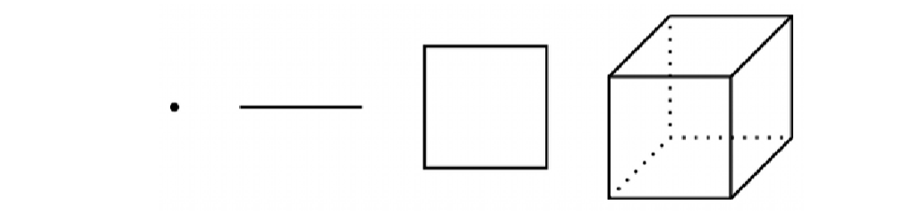
One might ask — can we consider higher dimensions?
The array is the natural extension of the vector and matrix, and can be extended to arbitrarily large $k$ dimensions:

\[ n_1 \times n_2 \times ... \times n_k. \]

Defining Arrays

Don’t get too excited!

In PSTAT 10 we only consider up to 3-dimensional arrays.
We can create an array using the array() function, which has similar arguments to the matrix() function:

# defining an array
array(data = NA,
      dim = length(data),
      dimnames = NULL)

The arguments of the array() function are:
- data — the input data (scalar, vector, matrix)
- dim — array dimensions (vector)
- dimnames — array dimension names (list)

Example — Defining Arrays

We can define a $2\times 2 \times 2$ array using the following code:

# define rubiks_cube array
rubiks_cube <- array(data = 1:8, dim = c(2, 2, 2))
rubiks_cube

, , 1

     [,1] [,2]
[1,]    1    3
[2,]    2    4

, , 2

     [,1] [,2]
[1,]    5    7
[2,]    6    8

Indexing extends naturally from matrices: instead of $(i,j)$ we now index with $(i,j,k)$, one subscript per dimension:

# element in row 1, column 2, slice 2
rubiks_cube[1, 2, 2]

[1] 7

You can see how this can naturally be extended to higher dimensions.
- Just be aware of the exponential growth in the number of elements as the number of dimensions increases.

🔁 Functions Over Arrays

We can apply operations (mathematical operations, functions) over an array using the apply() function:

# apply function
apply(X = array_object,
      MARGIN = array_margin,
      FUN = f)

X — the array object on which we are applying our operation
MARGIN — vector giving the subscripts for which the function will be applied over
FUN — function to be applied

For example, summing over MARGIN = 3 collapses each $2\times 2$ slice of rubiks_cube into a single total:

apply(X = rubiks_cube, MARGIN = 3, FUN = sum)

[1] 10 26

💪 Exercise — Constructing Arrays

03:00

For the next 3 minutes create a basic array to represent the faces of a solved two-color Rubik’s cube (each color appears on 3 of the cube’s six faces).

Define the matrices red and blue as $3 \times 3$ matrices where all entries are the character "r" and "b" respectively.
Construct an array using the red and blue matrices that represents the faces of the solved cube.

Hint: one of your array dimensions should refer to the cube’s 6 faces.

✅ Solution — Constructing Arrays

Define the Face Matrices

red <- matrix(rep("r", 9), nrow = 3, ncol = 3)
blue <- matrix(rep("b", 9), nrow = 3, ncol = 3)

Assemble the Cube

Stack 3 copies of red and 3 copies of blue along a third dimension representing the cube’s 6 faces:

rubiks_faces <- array(c(rep(red, 3), rep(blue, 3)), dim = c(3, 3, 6))

rubiks_faces[, , 1]
rubiks_faces[, , 6]

     [,1] [,2] [,3]
[1,] "r"  "r"  "r" 
[2,] "r"  "r"  "r" 
[3,] "r"  "r"  "r"

     [,1] [,2] [,3]
[1,] "b"  "b"  "b" 
[2,] "b"  "b"  "b" 
[3,] "b"  "b"  "b"

Lists

🗂️ What is a List?

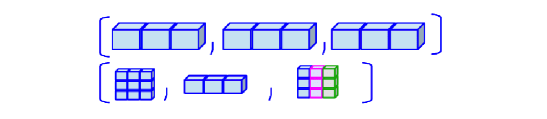
Lists are a flexible data structure that can contain multiple data types and even multiple data structures.
- They are similar to dictionaries in Python.
Each element of a list can be named and accessed using the $ operator.
What we gain in flexibility we lose in computational efficiency and mathematical tractability.
- Only numeric data types with regular structure (vectors, matrices, arrays) can be used in mathematical operations.

Example — Lists

To construct an example list we first define three objects to store: (1) a character vector; (2) a numeric matrix; and (3) a logical scalar.

# construct a list
list_example <- list(c("a", "b", "c"), matrix(data = 1:4, nrow = 2, ncol = 2), TRUE)
list_example

[[1]]
[1] "a" "b" "c"

[[2]]
     [,1] [,2]
[1,]    1    3
[2,]    2    4

[[3]]
[1] TRUE

Just like naming vector elements, we can name list elements using the names() function:

names(list_example) <- c("letters", "numbers", "flag")
list_example

$letters
[1] "a" "b" "c"

$numbers
     [,1] [,2]
[1,]    1    3
[2,]    2    4

$flag
[1] TRUE

🔓 Indexing Lists

The key difference between indexing lists and the other data types we have considered is that to index list elements we use double braces list_example[[...]].

list_example[[2]]
list_example[[3]]

     [,1] [,2]
[1,]    1    3
[2,]    2    4

[1] TRUE

If a list has named elements we can also index by name using the $ operator:

list_example$numbers
list_example$flag

     [,1] [,2]
[1,]    1    3
[2,]    2    4

[1] TRUE

Summary

✅ Topics Covered

🤔 Today we studied lots and lots of topics:

Matrices
Matrix Operations
Indexing
Arrays
Lists

📅 Next Class

🤩 Next class we continue our introduction by exploring multi-dimensional datatypes including:

Functions
Branching
Loops
Control Flow

PSTAT 10 Data Science Principles

Introduction

🔁 Review: Lecture 2

👀 Outline: Lecture 3

Matrices

🔢 What is a Matrix?

📐 Dimensionality

Dimension

Matrix Properties

matrix() Function

Example — matrix() Function

🪞 Transpose

🏷️ Row & Column Names

cbind() & rbind() Functions

Other ways to define matrices

🆔 Identity Matrix

Indexing Matrices

🎯 Indexing Matrices

Recall Vector Indexing

Matrix Indexing

Example — Indexing Matrices

Remember Matrix 1?

Indexing Example

🔪 Slicing Matrices

Sounds dramatic!

Submatrices

✂️ Removing Matrix Values

💪 Exercise — Matrix Construction

✅ Solution — Matrix Construction

Define the Matrix

Select the 3rd Row

Select Rows 3–5, Columns 1–3

Determine the Dimensions

Matrix Operations

🧮 Matrix Operations

Arrays

🧊 What are Arrays?

Moving into higher dimensions!

Defining Arrays

Don’t get too excited!

Example — Defining Arrays

🔁 Functions Over Arrays

💪 Exercise — Constructing Arrays

✅ Solution — Constructing Arrays

Define the Face Matrices

Assemble the Cube

Lists

🗂️ What is a List?

Example — Lists

🔓 Indexing Lists

Summary

✅ Topics Covered

📅 Next Class

`matrix()` Function

Example — `matrix()` Function

`cbind()` & `rbind()` Functions