Classification Models

This project was completed as part of the requirements for the course PSTAT231 Machine Learning taught by Prof. Coburn at the University of California Santa Barbara.

Introduction

In this project we compare supervised classification models for predicting forest cover type from cartographic features. We consider the following 6 classification methodologies:

• (Elastic Net) Multinomial Logistic Classification,
• K-Nearest Neighbors,
• (Pruned) Decision Trees,
• Random Forests,
• Gradient Boosted Decision Trees,
• Support Vector Machines.

We conduct our analysis in R using the tidymodels framework. Throughout this notebook we shall make use of the following packages:

# Libraries
library(tidyverse)
library(tidymodels)
library(kableExtra)
library(naniar)
library(psych)
library(GGally)
library(corrplot)
library(plotly)
library(gridExtra)
library(rpart.plot)
library(vip)
library(kernlab)

We first provide an outline of our chosen models in Section 2 before proceeding to discuss our data selection, preparation and exploration in ?@sec-data. Next, we detail our model training methodology in Section 5 before evaluating and comparing our models performace in Section 6. Finally, we conclude with a discussion of our results and potential future work in Section 7.

Methodology

Elastic Net Multinomial Logistic Classification

In statistics, the logistic model (or logit model) is a statistical model that models the probability of an event taking place by having the log-odds for the event be a linear combination of one or more independent variables. Formally, in binary logistic regression there is a single binary dependent variable, coded by an indicator variable, where the two values are labeled “0” and “1”, while the independent variables can each be a binary variable (two classes, coded by an indicator variable) or a continuous variable (any real value).

Multinomial logistic regression is a classification method that generalizes logistic regression to multiclass problems, i.e. with more than two possible discrete outcomes. Denote our categorical variable \(Y\) with levels \(\{1, ..., J\}\) and our predictors \(X_1, ..., X_p\). Multinomial logistic regression models the probability of each level \(j\) of \(Y\) by

\[ p_j(x):=\frac{e^{\beta_{0j}+\beta_{1,j}X_1+...+\beta_{pj}X_p}}{1+\sum_{l=1}^{J-1}e^{\beta_{0l}+\beta_{1l}X_1+...+\beta_{pl}X_p}} \]

for \(j=1, ..., J-1\) and

\[ p_J(x):=\frac{1}{1+\sum_{l-1}^{J-1}e^{\beta_{0l}+\beta_{1l}X_1+...+\beta_{pl}X_p}} \]

which implies that \(\sum_{j=1}^J p_j(x)=1\) and that there are \((J-1)\times(p+1)\) coefficients.

Typically, logistic regression analysis is performed using either the least absolute shrinkage and selection operator (lasso) method or ridge regression, each of which have their shortcomings. For our analysis we shall be using elastic net logistic regression which uses penalties from both the lasso and ridge regression techniques to learn from the shortcomings of each in an attempt to regularize our regression.

K-Nearest Neighbor Algorithm

The k-nearest neighbour (KNN) algorithm is a non-parametric supervised learning method used for both classification and regression. The input consists of the \(k\)-closest training examples in a data set and (in classification) the output is a class membership where an object is classified by a plurality vote of its neighbors with the object being assigned to the class most common among its \(k\) nearest neighbours.

Support Vector Machines

Support vector machines (SVM) are supervised learning models with associated learning algorithms. Given a set of training examples, each marked as belonging to one of two categories, an SVM training algorithm builds a model that assigns new examples to one category or the other, making it a non-probabilistic binary linear classifier. SVM maps training examples to points in space so as to maximise the width of the gap between categories. New examples are then mapped into that same space and predicted to belong to a category based on which side of the gap they fall.

(Pruned) Decision Tree

A decision tree is a non-parametric supervised learning algorithm which is utilized for both classification and regression tasks. It has a hierarchical structure consisting of a root node, branches, internal notes and lead nodes. Decision tree learning employs a divide and conquer strategy by conducting a greedy search to identify the optimal split points within a tree. This process of splitting is then repeated in a top-down, recursive manner until all, or the majority of records have been classified under specific class labels. A well known downside to decision trees is that as they grow in complexity they have a tendancy to overfit and compromise predictive power.

Pruning is a data compression technique that reduces the size of decision trees by removing sections of the tree that are non-critical and redundant to classify instances. Pruning reduces the complexity of the final classifier and hence improves predictive accuracy by the reduction of over fitting.

Gradient boosting is a machine learning technique used in regression and classification tasks whereby a prediction model is given in the form of an ensemble of weak prediction models, typically decision trees. When a decision tree is the weak learner, the resulting algorithm is called gradient-boosted trees and generally should outperform random forests.

Random Forests

Random forests are an ensemble learning method for classification (or regression) which operates by constructing a multitude of decision trees at training time. By growing numerous decision trees the model is able to classify a new object from an input vector, putting the input vector down each of the trees in the forest. Each tree gives a classification and we say the tree “votes” for that class then, the forest chooses the classification having the most votes (over all the trees in the forest).

Data Preparation

Data Source

Our data set containing real world data on forest cover type for various 30 x 30 meter cells and their corresponding cartographic variables for a study area consisting of four wilderness areas located in the Roosevelt National Forest of northern Colorado. These areas represent forests with minimal human-caused disturbances, so that existing forest cover types are more a result of ecological processes rather than forest management practices.

Our data set was prepared and published on Kaggle with the cover type information being collected from US Forest Service (USFS) Region 2 Resource Information System data and the predictors from data obtained from the US Geological Survey and USFS. The data set was provided pre-split into a training set - consisting of 15,120 observations with data for both predictors and the dependent variable - and a testing set - consisting of the remaining 565,892 observations with predictor data only.

We conduct this project throughout as if we were an initial contestant in the Kaggle competition in that we ensure that we fit and select models using only the provided training data set using no information from the testing data set. We also confirm that we won’t revisit this section once we have evaluated our model performance using the testing data.

We load our data as tree_train and inspect the shape.

# Import data
tree <- read.csv("data/covtype.csv")
tree_dim = dim(tree)
# Inspect dimensions of data frame
cat("Rows: ", tree_dim[1], "\nColumns: ", tree_dim[2])

Rows:  581012 
Columns:  55

Labels and Types

Inspecting the column names we see that we have multiple dummy variables for wilderness areas and soil types. We also have a number of continuous predictors such as elevation, aspect, slope, etc. Finally, we have our dependent variable Cover_Type which is a categorical variable with 7 levels corresponding to the 7 different forest cover types.

# Function to count number of columns containing a pattern
count_cols_containing <- function(df, pattern) {
  sum(grepl(pattern, names(df)))
}
# Count number of columns containing "Wilderness_Area" and "Soil_Type"
count_cols_containing(tree, "Wilderness_Area")

[1] 4

count_cols_containing(tree, "Soil_Type")

[1] 40

From the codebook provided with the data set, we see that each Soil_Type category actually contains two pieces of information, the soil family and details of the terrain. We therefore conclude our data preparation by splitting this column into two, naming them Soil_Family and Terrain, both of which are converted to factor variables. We save our prepared data as covtype_clean.csv - note that loading the data requires converting catagorical columns to factors.

# Creating wilderness area categorical variable
wilderness_index <- which(grepl("Wilderness", colnames(tree)))
wilderness_area_names <- c("Rawah",
                           "Neota",
                           "Comanche Peak",
                           "Cache la Poudre")
wilderness <- wilderness_area_names[max.col(tree[, wilderness_index])]

# Creating soil type categorical variable
soil_index <- which(grepl("Soil", colnames(tree)))
soil_type_names <- c("Cathedral family - Rock outcrop complex, extremely stony",
                           "Vanet - Ratake families complex, very stony",
                           "Haploborolis - Rock outcrop complex, rubbly.",
                           "Ratake family - Rock outcrop complex, rubbly.",
                           "Vanet family - Rock outcrop complex complex, rubbly.",
                           "Vanet - Wetmore families - Rock outcrop complex, stony.",
                           "Gothic family.",
                           "Supervisor - Limber families complex.",
                           "Troutville family, very stony.",
                           "Bullwark - Catamount families - Rock outcrop complex, rubbly.",
                           "Bullwark - Catamount families - Rock land complex, rubbly.",
                           "Legault family - Rock land complex, stony.",
                           "Catamount family - Rock land - Bullwark family complex, rubbly.",
                           "Pachic Argiborolis - Aquolis complex.",
                           "unspecified in the USFS Soil and ELU Survey.",
                           "Cryaquolis - Cryoborolis complex.",
                           "Gateview family - Cryaquolis complex.",
                           "Rogert family, very stony.",
                           "Typic Cryaquolis - Borohemists complex.",
                           "Typic Cryaquepts - Typic Cryaquolls complex.",
                           "Typic Cryaquolls - Leighcan family, till substratum complex.",
                           "Leighcan family, till substratum, extremely bouldery.",
                           "Leighcan family, till substratum - Typic Cryaquolls complex.",
                           "Leighcan family, extremely stony.",
                           "Leighcan family, warm, extremely stony.",
                           "Granile - Catamount families complex, very stony.",
                           "Leighcan family, warm - Rock outcrop complex, extremely stony.",
                           "Leighcan family - Rock outcrop complex, extremely stony.",
                           "Como - Legault families complex, extremely stony.",
                           "Como family - Rock land - Legault family complex, extremely stony.",
                           "Leighcan - Catamount families complex, extremely stony.",
                           "Catamount family - Rock outcrop - Leighcan family complex, extremely stony.",
                           "Leighcan - Catamount families - Rock outcrop complex, extremely stony.",
                           "Cryorthents - Rock land complex, extremely stony.",
                           "Cryumbrepts - Rock outcrop - Cryaquepts complex.",
                           "Bross family - Rock land - Cryumbrepts complex, extremely stony.",
                           "Rock outcrop - Cryumbrepts - Cryorthents complex, extremely stony.",
                           "Leighcan - Moran families - Cryaquolls complex, extremely stony.",
                           "Moran family - Cryorthents - Leighcan family complex, extremely stony.",
                           "Moran family - Cryorthents - Rock land complex, extremely stony.")
soil_type <- soil_type_names[max.col(tree[, soil_index])]

# Replace dummy variables with categorical (training data)
tree <- tree[,!(names(tree) %in% colnames(tree)[c(wilderness_index, soil_index)])]
tree["Wilderness"] <- wilderness
tree["Soil_Type"] <- soil_type

# Convert categorical variables to factors
tree$Wilderness <- as.factor(tree$Wilderness)
tree$Soil_Type <- as.factor(tree$Soil_Type)

# Convert dependent variable to categorical with labels
tree$Cover_Type = as.factor(tree$Cover_Type)
levels(tree$Cover_Type) = c("Spruce_or_Fir","Lodgepole_Pine",  "Ponderosa_Pine","Cottonwood_or_Willow",
                            "Aspen","Douglas_fir","Krummholz")
# Splitting soil type variable into terrain and soil family
terrain_names <- c("stony","stony","rubbly","rubbly","rubbly","stony","neither","neither","stony",
                   "rubbly","rubbly","stony","rubbly","neither","neither","neither","neither","stony",
                   "neither","neither","neither","neither","neither","stony","stony","stony","stony",
                   "stony","stony","stony","stony","stony","stony","stony","neither","stony","stony",
                   "stony","stony","stony")
soil_family_names = c("Cathedral","Ratake","Haploborolis","Ratake","Vanet","Vanet","Gothic","Limber",
                      "Troutville","Catamount","Catamount","Legault","Catamount","None","None","None",
                      "Gateview","Rogert","None","None","Leighcan","Leighcan","Leighcan","Leighcan",
                      "Leighcan","Catamount","Leighcan","Leighcan","Legault","Legault","Leighcan",
                      "Catamount","Leighcan","None","None","Bross","None","Leighcan","Moran", "Moran")
idx <- match(tree$Soil_Type, soil_type_names)
soil_family <- soil_family_names[idx]
terrain     <- terrain_names[idx]

# Assigning to data set
tree$Soil_Family = as.factor(soil_family)
tree$Terrain = as.factor(terrain)

# Create factors
tree$Cover_Type <- as.factor(tree$Cover_Type)
tree$Wilderness <- as.factor(tree$Wilderness)
tree$Soil_Type  <- as.factor(tree$Soil_Type)
tree$Soil_Family <- as.factor(tree$Soil_Family)
tree$Terrain <- as.factor(tree$Terrain)

Now we can inspect our prepared data which we see has 13 predictors for the dependent variable Cover_Type, 10 of which are continuous with 3 categorical variables (not including Soil_Type which we do not consider). We provide a summary of variables included in our cleaned data set below in Table 1.

Table 1: Model predictor descriptions

Variable	Unit	Description
Elevation	Meters	Elevation in meters
Aspect	Degrees Azimuth	Aspect in degrees azimuth
Slope Gradient	Degrees	Slope in degrees
Horizontal distance to hydrology	Meters	Horz Dist to nearest surface water features
Vertical distance to hydrology	Meters	Vert Dist to nearest surface water features
Horizontal distance to roadways	Meters	Horz Dist to nearest roadway
Hillshade 9am	Index (0-255)	Hillshade index at 9am, summer solstice
Hillshade Noon	Index (0-255)	Hillshade index at noon, summer solstice
Hillshade 3pm	Index (0-255)	Hillshade index at 3pm, summer solstice
Horizontal distance to fire points	Meters	Horz Dist to nearest wildfire ignition points
Wilderness Area	Cat	Wilderness area designation
Soil Family	Cat	Soil family categories: (1) Bross, (2) Catamount, (3) Cathedral, (4) Gateview, (5) Gothic, (6) Haploborolis, (7) Legault, (8) Leighcan, (9) Limber, (10), Moran, (11) None, (12) Ratake, (13) Rogert. (14) Troutville, (15) Vanet
Terrain	Cat	Terrain categories: (1) Stony, (2) Rubbly, (3) Neither.

Missingness Analysis

We first inspect the missingness of the data set by computing the cound and percentage of missing values for each column, summarized below in Table 2, and from which we see that there are no mssing values in our data.

# Count and percentage of missing values for each column
missing_summary <- tree %>%
  summarise_all(list(Count = ~sum(is.na(.)),
                     Percent = ~mean(is.na(.)) * 100)) %>%
  pivot_longer(cols = everything(),
               names_to = c("Variable", "Metric"),
               names_pattern = "^(.+)_(Count|Percent)$") %>%
  pivot_wider(names_from = Metric, values_from = value)
# Display missing summary table
kbl(missing_summary, caption = "Missingness summary for each variable in the data set") %>%
  kable_styling(full_width = FALSE, position = "center")

Table 2: Missingness summary for each variable in the data set

Variable	Count	Percent
Elevation	0	0
Aspect	0	0
Slope	0	0
Horizontal_Distance_To_Hydrology	0	0
Vertical_Distance_To_Hydrology	0	0
Horizontal_Distance_To_Roadways	0	0
Hillshade_9am	0	0
Hillshade_Noon	0	0
Hillshade_3pm	0	0
Horizontal_Distance_To_Fire_Points	0	0
Cover_Type	0	0
Wilderness	0	0
Soil_Type	0	0
Soil_Family	0	0
Terrain	0	0

Train and Test Split

We conduct this project throughout as if we were an initial contestant in the Kaggle competition in that we only consider the training data. We therefore split our file into our training and testing sets named tree_train and tree_test respectively. Throughout this project we shall employ hyperparameter tuning procedures - whereby we tune the value of our model input parameters - and so we also fold our data using the function vfold_cv.

# alternative data split matching initial project assignment
tree_train <- tree[1:15120, ]
tree_test <- tree[15120:dim(tree)[1], ]

# k fold cross validation
tree_fold <- vfold_cv(tree_train, v = 10)

Data Exploration

Response Variable Distribution

We examine the distribution of the dependent variable Cover_Type in our training data, shown below in Figure 1. We see clearly that the distribution of the response is balanced.

# count plot of cover type in training data
ggplot(tree_train, aes(x=Cover_Type, fill=Cover_Type)) +
  geom_bar(aes(Cover_Type), width=0.55) +
  scale_x_discrete(labels = function(x) str_replace_all(x, "_", " ")) +
  theme_minimal() +
  theme(axis.text.x = element_text(angle = 35, vjust = 1, hjust=1))+
  labs(x = "Tree Coverage Type", y = "Count", title = "Distribution of Cover Type in Training Data") +
  theme(legend.position = "none")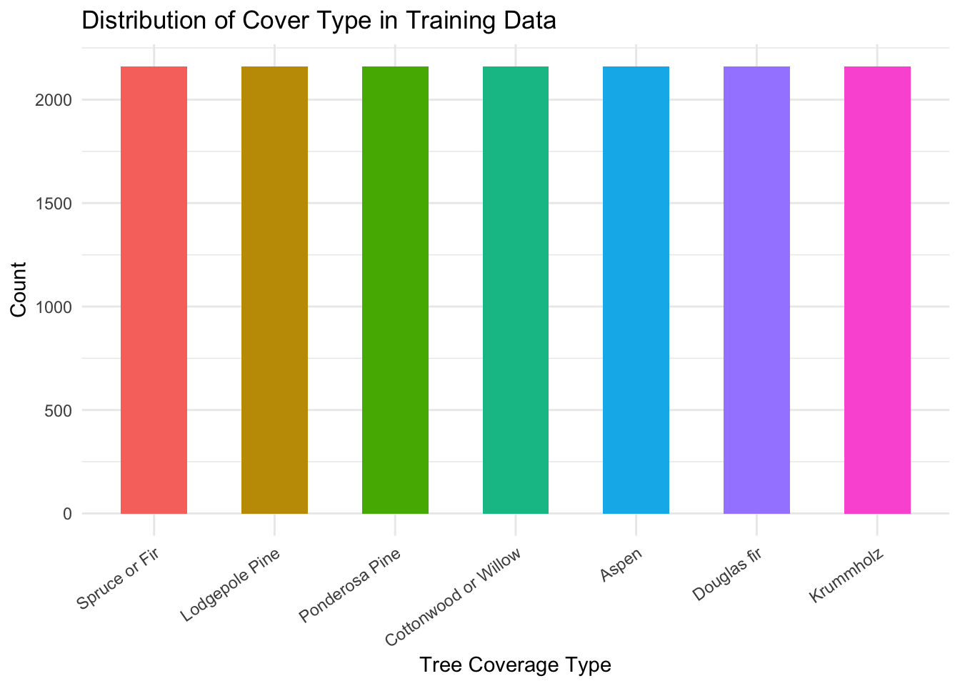

Figure 1: Count plot of dependent variable cover type in training data sample.

Univariate Distributions

We produce count plots for each of our three categorical predictors, Wilderness, Terrain and Soil_Family, grouped by Cover_Type, shown below in Figure 2, Figure 3 and Figure 4. We are inspecting for class separation in the distribution of our predictors across the levels of our response variable.

Wilderness

ggplot(data=tree_train, aes(x=Wilderness, fill=Cover_Type)) +
  geom_bar(aes(Wilderness), position = "fill", width=0.55) +
  scale_x_discrete(labels = function(x) str_replace_all(x, "_", " ")) +
  scale_fill_discrete(labels = function(x) str_replace_all(x, "_", " ")) +
  scale_y_continuous(labels = scales::percent) +
  theme_minimal() +
  theme(axis.text.x = element_text(angle = 90, vjust = 0.5, hjust=1))+
  labs(x = "Wilderness Area", y = "Proportion", title = "Distribution of Wilderness Area in Training Data", fill = "Cover Type")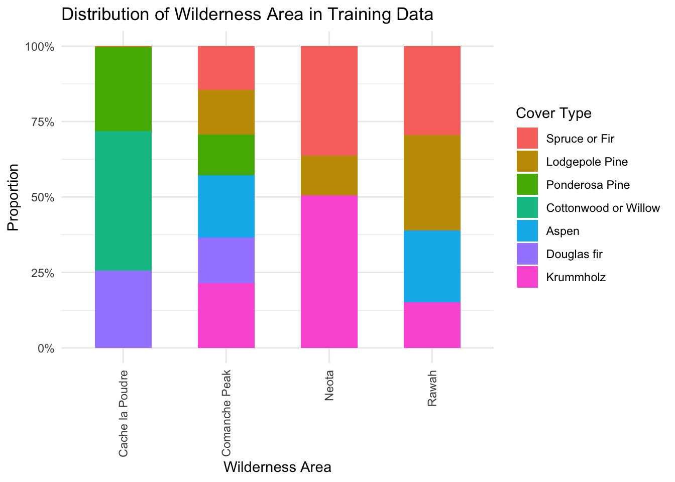

Figure 2: Count plot of wilderness area in training data sample grouped by cover type.

Terrain

ggplot(data=tree_train, aes(x=Terrain, fill=Cover_Type)) +
  geom_bar(aes(Terrain), position = "fill", width=0.55) +
  scale_x_discrete(labels = function(x) str_replace_all(x, "_", " ")) +
  scale_fill_discrete(labels = function(x) str_replace_all(x, "_", " ")) +
  scale_y_continuous(labels = scales::percent) +
  theme_minimal() +
  theme(axis.text.x = element_text(angle = 90, vjust = 0.5, hjust=1))+
  labs(x = "Terrain", y = "Proportion", fill = "Cover Type")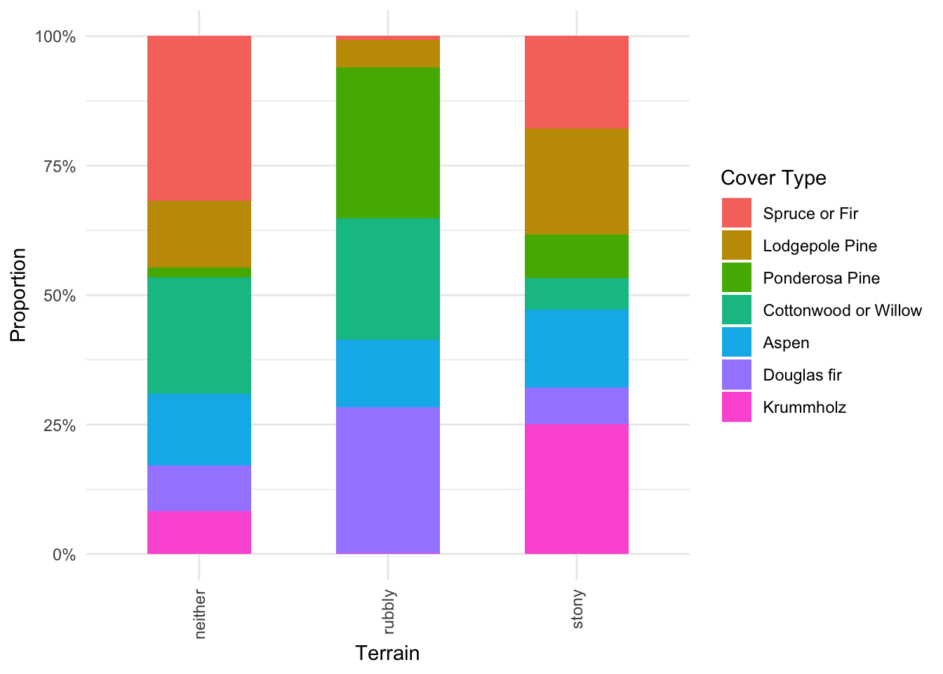

Figure 3: Count plot of terrain in training data sample grouped by cover type.

Soil Family

ggplot(data=tree_train, aes(x=Soil_Family, fill=Cover_Type)) +
  geom_bar(aes(Soil_Family), position = "fill", width=0.55) +
  scale_x_discrete(labels = function(x) str_replace_all(x, "_", " ")) +
  scale_fill_discrete(labels = function(x) str_replace_all(x, "_", " ")) +
  scale_y_continuous(labels = scales::percent) +
  theme_minimal() +
  theme(axis.text.x = element_text(angle = 90, vjust = 0.5, hjust=1))+
  labs(x = "Soil Family", y = "Proportion", fill = "Cover Type")

Figure 4: Count plot of soil family in training data sample grouped by cover type.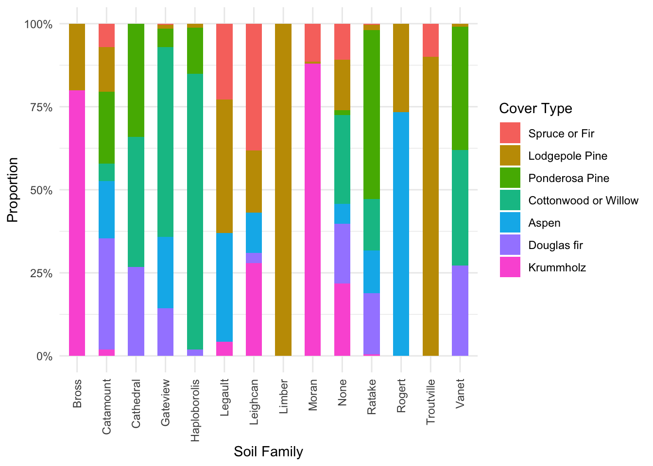

Moving onto explore our predictors we begin by producing a correlation plot of all 10 continuous predictors in the data set, shown below in Figure 5.

tree_train %>% 
  select(where(is.numeric)) %>% # selecting numeric columns
  cor() %>%
  corrplot(type = "lower", diag = FALSE)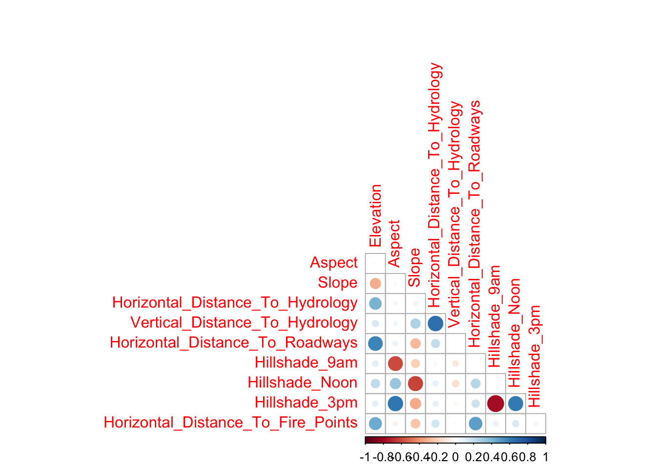

Figure 5: Correlation plot of numerical predictors in training data sample.

Note that for convenience when discussing our results we shall refer to individual plots in Figure @ref(fig:corrplot2) as \((i,j)\) where \(i\) is the row number and \(j\) is the column number. From our results we make the following initial observations which we aim to explore further:

• Elevation is showing evidence of being a strong predictor as the distribution plot \((1,1)\) is showing evidence of factor separation.

• In both Figure @ref(fig:corrplot1) and see evidence of significant correlation between all three Hillshade variables, indicating the potential need for interaction terms.

• Furthermore, we see evidence of correlation between the Hillshade variables and both Aspect and Slope, a reasonable finding as Hillshade is likely to be influenced by both of these factors.

• Finally, we see a significant correlation between Horizontal_Distance_To_Hydrology and Vertical_Distance_To_Hydrology, again a reasonable finding as the further a test area is away from Hydrology the more likely it has to have significant elevation change.

Exploring these observations further we produce a plot examining the empirical distribution of Elevation split into groups based on Cover_Type, shown below in Figure @ref(fig:elevation). As mentioned in our initial observation of the correlation plots, there is significant class separation indicating that Elevation might contain powerful predictive information.

ggplot(tree_train, aes(x=Elevation, split=Cover_Type, fill=Cover_Type)) + 
  geom_density(alpha=0.5) + 
  theme_minimal()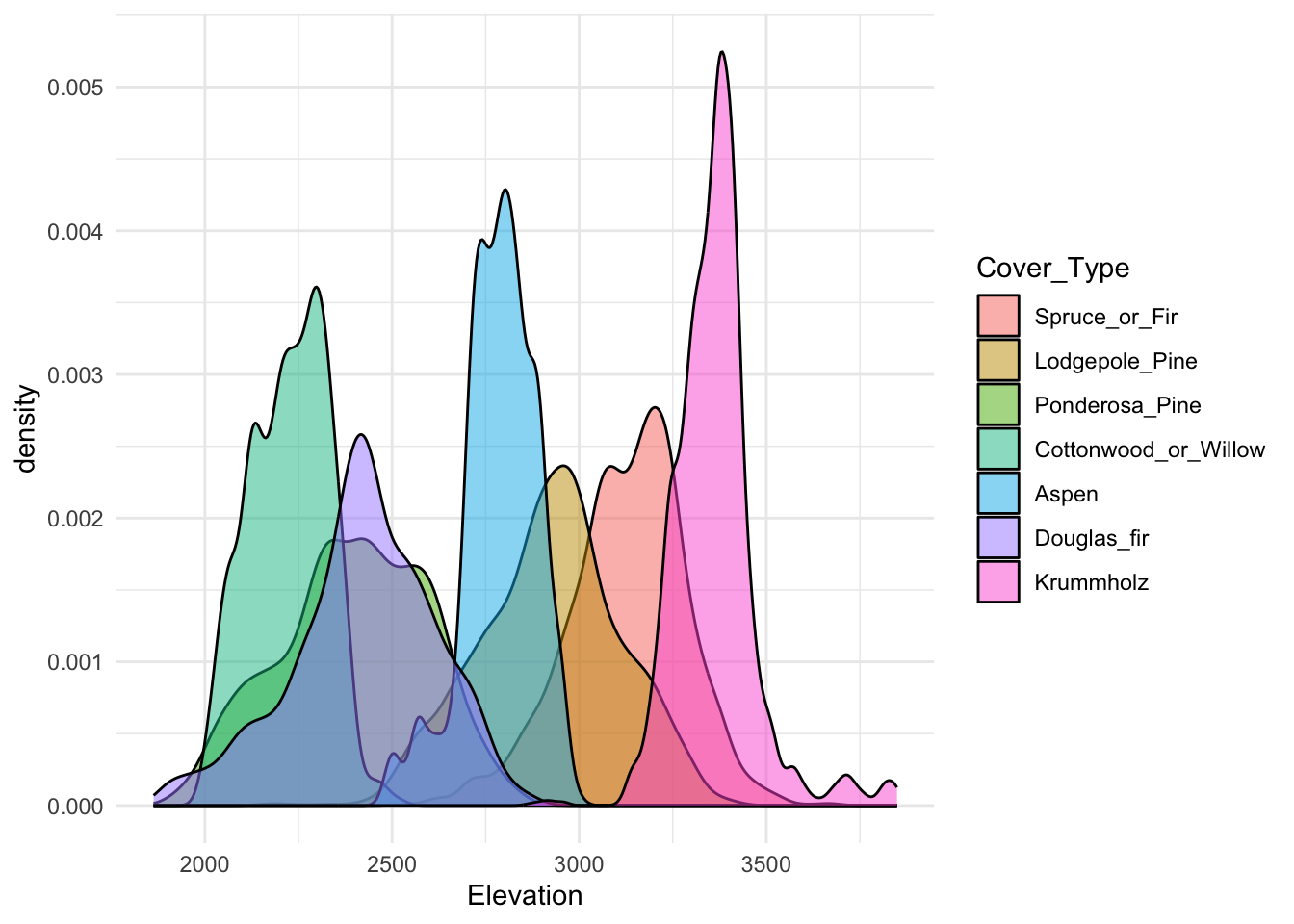

Distribution plot of elevation split by coverage type.

We conclude our exploration of our continuous predictors by producing a 3D plot examining the relationship between Slope, Elevation and Hillshade_9am, shown below in Figure @ref(fig:elevationthree).

plot_ly(x=tree_train$Elevation, y=tree_train$Slope, z=tree_train$Hillshade_9am, type="scatter3d", mode="markers", color=tree_train$Cover_Type)

3-D scatter plot of Elevation, Slope and Hillshade 9am variables.

This plot is very useful as it shows some highly significant class separation as a result on considering these three variables simultaneously, indicating that there variables will likely provide a significant role in our models.

Training

Evaluation

Conclusion