Code
# Packages
import numpy as np
import matplotlib.pyplot as plt# Packages
import numpy as np
import matplotlib.pyplot as pltLet \(\{\xi_n\}_{n\in\mathbb{N}}\) where \(\xi_n:=(\xi_n^{(1)}, ..., \xi_n^{(m)})\) be a sequence of independent and identically distributed random vectors taking values in \(\mathbb{R}^m\). An \(m\)-dimensional random walk (RW) \(\{S_n\}_{n\in\mathbb{N}_0}\) is defined by the recursive expression
\[ \begin{cases} S_n = S_{n-1} + \xi_{n} & n\in\mathbb{N}\\ S_0 = s_0\in\mathbb{R}^m. \end{cases} \]
Through repeated substitution we quickly obtain the closed form expression
\[ S_n = S_0 + \sum_{i=1}^n\xi_i. \]
If \(\mathbb{P}(\xi_n^{(j)}=1)=p=1-\mathbb{P}(\xi_n^{(j)}=-1)\) for all \(n,j\) then the RW is said to be simple. Furthermore, if \(p=\frac{1}{2}\) then the RW is said to be symmetric.
Unless otherwise stated in this note we assume that \(m=1\).
Example: We specify that \(\xi_i\stackrel{\text{i.i.d.}}{\sim}\text{Normal}(0,1)\) and \(S_0=0\). We can simulate a realization \(\{S_j\}_{j=1}^{n}\) of length \(n=1000\) using the python code below:
def normal_RW(mu=0, sigma=1, s0= 0, n=1000):
    xi = np.random.normal(loc=0, scale=1, size=n)
    s = np.concatenate([[s0], s0 + np.cumsum(xi)])
    return s
np.random.seed(42)
S1 = normal_RW()
plt.figure(figsize=(8, 4))
plt.plot(S1)
plt.xlabel(r"$n$")
plt.ylabel(r"$S_n$")
plt.title(r"Gaussian random walk $\{S_n\}$ of length $n=1000$.")
plt.show()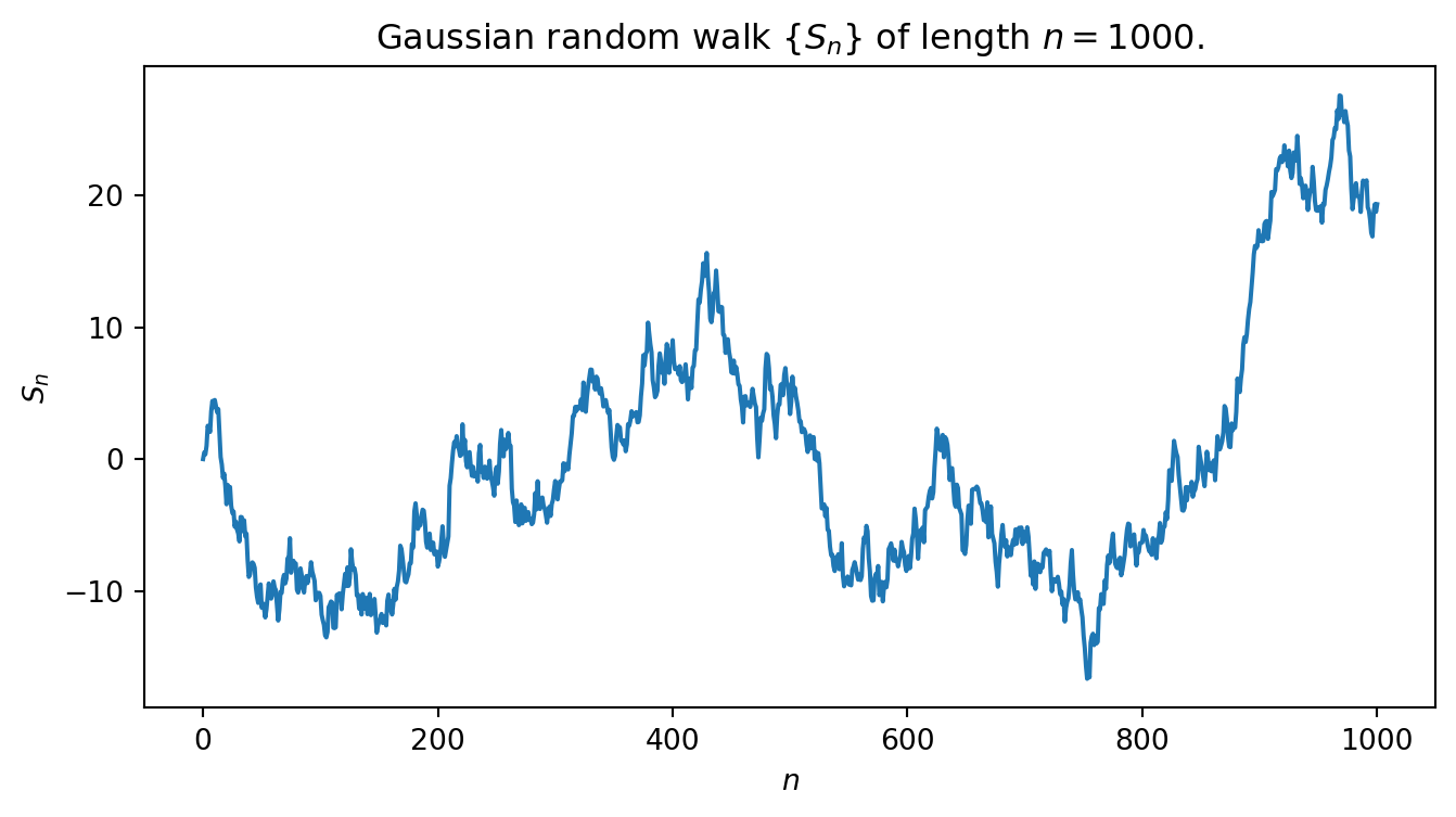
For a simple RW \(\{S_n\}\)
\[ \mathbb{P}(S_n-S_0=k) = \begin{cases} {n \choose \frac{n+k}{2}}p^{\frac{n+k}{2}}(1-p)^{\frac{n-k}{2}} & n+k\text{ is even} \\ 0 & \text{otherwise}.\end{cases} \]
Proof:
Without loss of generality assume that \(k>0\) and denote the number of upwards steps by \(u\). To reach state \(k\) in \(n\) steps we must therefore have that
\[ u + (n-) \]