P = np.array([
    [.4, .6, 0],
    [.7, .3, 0],
    [0, .1, .9]
])
P3 = np.linalg.matrix_power(P,3); print(P3)
[[0.526 0.474 0. ]
[0.553 0.447 0. ]
[0.112 0.159 0.729]]In probability theory a stochastic process is said to satisfy the Markov property if its future evolution is independent of its history, that is, the process is memoryless. Consider a discrete time stochastic process \(\{X_t\}_{t\in\mathbb{N}}\) defined in the probability space \((\Omega,\mathcal{F}, \mathbb{P})\).
Definition: (Markov Property)
The discrete time stochastic process \(\{X_t\}_{t\in\mathbb{N}}\) is said to satisfy the Markov property if \[\mathbb{P}(X_{n+1}=x_{n+1}|X_n=x_n, ..., X_1=x_1)=\mathbb{P}(X_{n+1}=x_{n+1}|X_n=x_n).\]
Intuitively, we see that we gain no additional information about the probability of the next value of the process by conditioning on the entire history rather than the latest value. Any process satisfying the markov property is called a Markov process.
A Markov process with a discrete state space is known as a Markov chain (MC). Assume that \(\{X_t\}_{t\in\mathbb{N}}\) is a Markov chain with finite state space \(\mathcal{X}:=\{1, ..., M\}\). The evolution of the chain in time is described by transition probabilities \(p_{i,j}^{(n)}(t)\) which give the probability that the chain is in state \(j\) at time \(t+n\) given that the chain was in \(i\) at time \(t\) \[ p_{i,j}^{(n)}(t)=\mathbb{P}(X_{t+n}=j|X_{t}=i). \]
We summarize the transition probabilities in an \(M\times M\) transition probability matrix denoted by \[ P^{(n)}(t)=(p_{i,j}^{(n)}(t))_{i,j\in\mathcal{X}}. \]
The transition probability matrix is stochastic which means that for all \(n,t\in\mathbb{N}\) we have:
To simplify notation we denote the one-step transition probablity matrix
\[
P(t)=(p_{i,j}(t))_{i,j\in\mathcal{X}}.
\]
The transition probabilities are stationary when they are invariant in time, that is \[ p_{i,j}^{(n)}(t)=p_{i,j}^{(n)}(s);~~\forall s,t\in\mathbb{N}. \]
We say that a MC is homogenous if it has stationary transition probabilities. For homogenous MCs we are often interested in the one-step transition probabilities and so again to clarify notation we denote the one-step transition probability matrix for homogenous MCs as \[ P=(p_{i,j})_{i,j\in\mathcal{X}}. \]
Example: Consider a homogenous MC \(\{X_t\}\) with finite state space \(\mathcal{S}:=\{1,2,3\}\) with transition probability matrix \[ P = \begin{bmatrix} 0 & 0.6 & 0.2 & 0.2 \\ 0.75 & 0 & 0.25 & 0 \\ 0.25 & 0.25 & 0.25 & 0.25 \\ 0.25 & 0 & 0.25 & 0.5 \end{bmatrix}. \]
To gain deeper insight into the behavior of the chain we typically will produce transition probability diagram which takes the form of a directed graph with nodes denoting states and weighted directed arrows the transition probabilities. The transition probability diagram for our example is
![]()
There are several alternate versions of this diagram including the integer weighted diagram. To construct the integer-weighted diagram we compute the inter-weighted matrix by multiplying elements of each row by the lowest common multiple for that row. The integer weighted matrix for our example is \[ P = \begin{bmatrix} 0 & 3 & 1 & 1 \\ 3 & 0 & 1 & 0 \\ 1 & 1 & 1 & 1 \\ 1 & 0 & 1 & 2 \end{bmatrix}. \]
The corresponding diagram is
![]()
Since our diagram has a symmetric integer-weighted transition matrix we can also write the non-directed version by combining the equally weighted directed arrows into a single non-directed line
![]()
The state distribution \(\mu_i(t)\) gives the probability that the chain is in state \(i\) at time \(t\) \[ \mu_i(t)=\mathbb{P}(X_{t}=i). \]
For convenience we summarize the state distributions in vector notation \[ \boldsymbol{\mu}(t)=(\mu_i(t))_{i \in \mathcal{X}}. \]
Of particular interest is the initial state distribution \[ \boldsymbol{\mu}(0)=\boldsymbol{\mu}=(\mu_i(0))_{i \in\mathcal{X}}. \]
For conveinence we also introduce the following notation for process vectors \[ X_{1:t} = (X_1, ..., X_t), \]
where similarly \(X_{1:t}=x_{1:t}\) is equivalent to \(X_1=x_1, ..., X_t=x_t\).
Finite-dimensional distributions allow us to evaluate the behavior of the distribution of infinite length processes by selecting some sub-sequence of index values to evaluate their joint distribution.
Proposition (Finite-Dimensional Distributions):
The finite-dimensional distributions of \(X=(X_{n})_{n}\) are determined by the initial mass \(\mu^{(0)}\) and transition matrix \(P\) where \[P(X_{0}=i_{0}, \dots, X_{n}=i_{n})=\mu_{{x_{0}}}^{(0)}p_{x_{0}, x_{1}}(0)p_{x_{1}, x_{2}}(1)\cdots p_{x_{n-1}, x_{n}}(n-1).\]
Proof:
From application of the Chain Rule and the Markov Property we see that \[
\begin{align}
\mathbb{P}&(X_{1 : n}=x_{1: n}) & \\
& = \mathbb{P}(X_{0}=x_{0}) \mathbb{P}(X_{1}=x_{1}|X_{0}=x_{0})\mathbb{P}(X_{2}=x_{2}|X_{0 : 1}=x_{0 : 1})\cdots \\
& \quad \cdots \mathbb{P}(X_{n}=x_{n}|X_{0 : n-1}=x_{0: n-1}) \\
& =\mathbb{P}(X_{0}=x_{0})\mathbb{P}(X_{1}=x_{1}|X_{0}=x_{0})\mathbb{P}(X_{2}=x_{2}|X_{1}=x_{1})\cdots \\
& \quad \cdots \mathbb{P}(X_{n}=x_{n}|X_{n-1}=x_{n-1}) \\
& = \mu_{{x_{0}}}^{(0)}p_{x_{0}, x_{1}}(0)p_{x_{1}, x_{2}}(1)\cdots p_{x_{n-1}, x_{n}}(n-1),
\end{align}
\]
as required.
\(\square\)
Proposition: (Multi-step Transition Probabilities for homogenous MCs)
Let \(\{ X_{n} \}\) be a homogenous MC with one-step transition probability matrix \(P\). The \(m\)-step transition probabilities are given by raising the one-step transition probability matrix to the \(m\)-th power \[P^{(m)}=(\mathbb{P}(X_{m}=j|X_{0}=i))_{i,j}=P^m.\]
Proof:
The result follows immediately from the Markov property since \[
\begin{aligned}
\mathbb{P}(X_{m}|X_{0}) & =\mathbb{P}(X_{m}|X_{m-1})\mathbb{P}(X_{m-1}|X_{0}) \\
& = \qquad \vdots \\
& = \mathbb{P}(X_{m}|X_{m-1})\cdots \mathbb{P}(X_{1}|X_{0}) \\
& = [\mathbb{P}(X_{1}|X_{0})]^m.
\end{aligned}
\]
\(\square\)
Example 1: Consider a homogenous MC with state space \(\mathcal{S}:=\{ 1,2,3 \}\) with transition probability matrix \(P\) and initial state distribution \(\mu\) given respectively by \[ P:=\begin{bmatrix} 0.4 & 0.6 & 0 \\ 0.7 & 0.3 & 0 \\ 0 & 0.1 & 0.9 \end{bmatrix},~~\mu=\begin{bmatrix} 0.1 & 0.2 & 0.7 \end{bmatrix}. \]
The transition probability diagram for this chain is
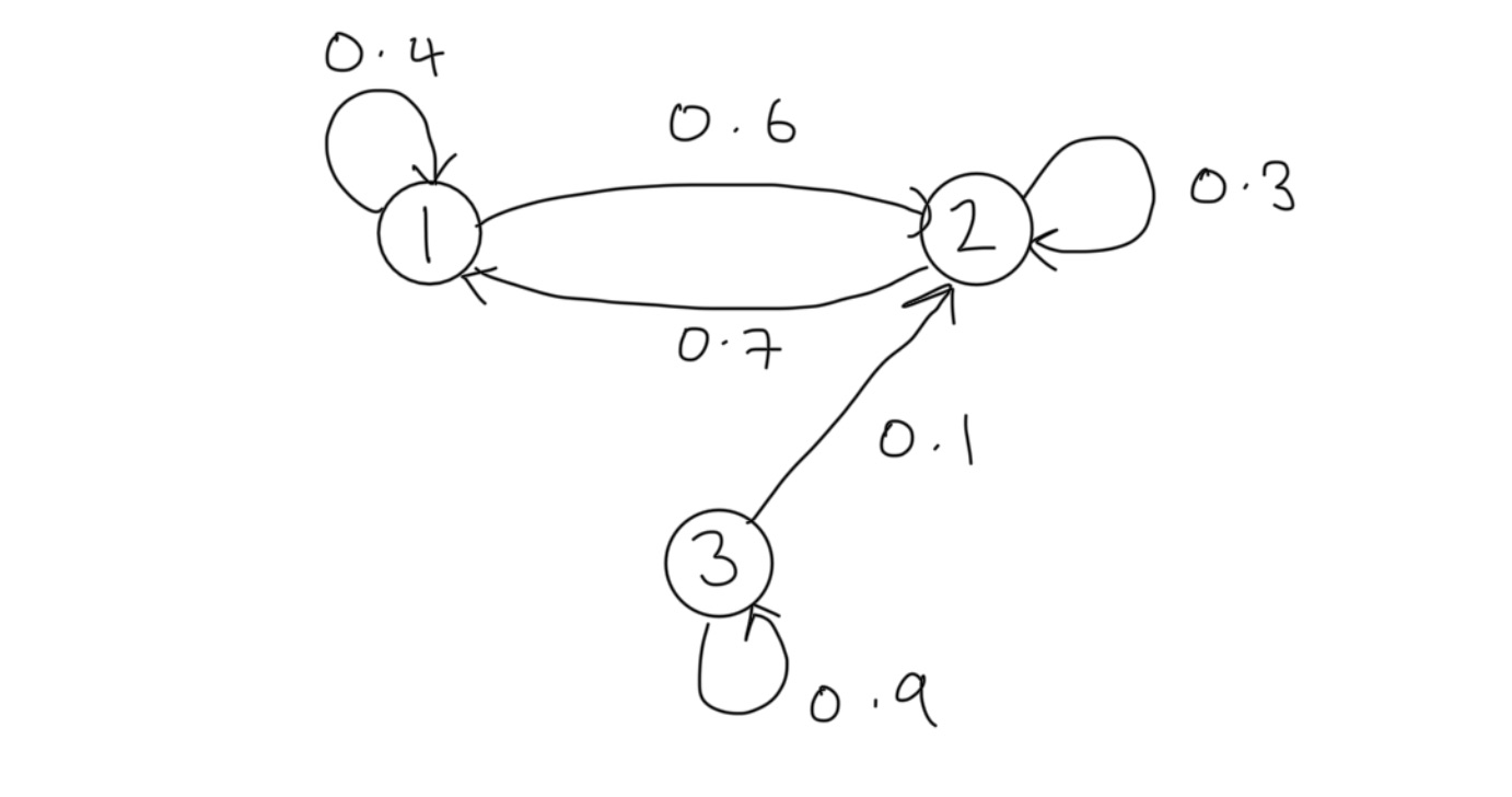
Suppose we wish to determine the \(3\)-step transition probabilities. Applying Proposition 1 we can compute \(\mathbb{P}(X_3|X_0)\) as \(P^3\):
P = np.array([
[.4, .6, 0],
[.7, .3, 0],
[0, .1, .9]
])
P3 = np.linalg.matrix_power(P,3); print(P3)[[0.526 0.474 0. ]
[0.553 0.447 0. ]
[0.112 0.159 0.729]]Furthermore, let us suppose that we wish to determine the 3-step state distribution. From the finite-dimensional distribution we see that \[ \begin{aligned} \mathbb{P}(X_3) & =\mathbb{P}(X_0)\mathbb{P}(X_1|X_0)\mathbb{P}(X_2|X_1)\mathbb{P}(X_3|X_2) \\ & = \boldsymbol{\mu}P^3. \end{aligned} \]
Thus we can compute:
mu = np.array([
    0.1, 0.2, 0.7
])
mu@(P3)
array([0.2416, 0.2481, 0.5103])
We can classify MC states based on how they appear in the chain and their behavior in the limit. States can be persistent (recurrent), null-persistent, transient, absorbing, periodic and ergodic.
Definition: (Persistent States) A state \(j\) is persistent if the probability that the process will return to \(j\) given that it started at \(j\) eventually is 1, that is \[\mathbb{P}(X_{n}=j~\text{for some}~n\geq 1|X_{0}=j)=1.\]
A sub-class of persistent states are null-persistent states which are persistent thats that have an infinite mean recurrence time. States that are not null-persistent are said to be positive_persistent.
For example, consider a symmetric random walk. Any point in the state space is null-persistent since the random walk can always return but may take infinitely long to do so. We discuss null-persistent states in a later note on MCs.
Definition: (Transient States)
Alternatively, if a state \(j\) is not persistent it must be transient, that is, the probability that the process will return to \(j\) given that it started at \(j\) eventually is 0 i.e. the processes structure prevents it from returning. This is equivalent to writing \[\mathbb{P}(X_{n}=i~\text{for some}~n\geq 1|X_{0}=i)<1.\]
Definition: (Periodic States)
The period of a state \(j\) is the greatest common divider of all \(n\) for which \(p_{{i,i}}(n)>0\) i.e. \[d(i)=gcd\{n:p_{i,i}(n)>0\}.\] If \(d(i)=1\) then the state \(j\) is aperiodic and otherwise, the state is said to be periodic.
Definition: (Ergodic)
A state \(j\) is ergodic if it is positive persistent and aperiodic i.e. \(\mu_{i,i}<\infty\) and \(d(i)=1\).
Definition: (Absorbing)
A state \(j\) is absorbing if \(p_{j,j}=1\), that is the probability of leaving state \(j\) once the process has entered is 0.
To classify chains we first define state communication, that is when paths between states have non-zero probability.
Definition: (Communicating States)
For MC \(\{ X_{t} \}\) state \(i\) communicates with state \(j\), denoted \(i \to j\), if \(p_{i,j}(n)>0\) for some \(n\). If \(i\to j\) and \(j \to i\) we say that \(i\) and \(j\) intercommunicate, denoted \(i \leftrightarrow j\).
We can show that intercommunication is an equivalence class and thus can be used to split MC state spaces into communication classes. For \(i,j\) in the same communication class we have:
States \(i\) and \(j\) have the same period;
State \(i\) is transient iff \(j\) is transient; and
State \(i\) is null persistent iff \(j\) is.
Definition: (Irreducibility)
A set of states \(C\) is irreducible if for all \(i,j\in C\), \(i\leftrightarrow j\), that is all states within \(C\) inter-communicate.
Definition: (Closed)
A set of states \(C\) is closed if for all \(i \in C\), \(p_{i,j}=0\) for all \(j\not\in C\), that is, the chain never leaves \(C\) once it has entered. Not that clearly the set consisting of one absorbing state is closed.
Example: Consider the MC transition diagram shown in the figure below.
![]()
We define \(S_1:=\{5\}\), \(S_2:=\{1,2,3,4\}\) and \(S_3:=\{6,7\}\). The chain is clearly reducible since \(2\to 5\) and \(3\to 6\) are one way journies. We can see that \(5\) is absorbing since the chain can never leave once it arrives. We see that states \(1,2,3,4\) are transient since the chain will visit them and never return at some point, and states \(6\) and \(7\) are recurrent since the chain will always revisit them. We say that \(S_1\) is an closed recurrent (absorbing) class, \(S_2\) is a transient class and \(S_3\) is a closed recurrent class.
The Chapman-Kolmogorov Equations (CKE) relate the joint probability distributions of different sets of coordinates on a stochastic process.
Theorem 2: (Chapman-Kolmogorov Equations)
For a discrete time countable state homogeneous Markov chain the Chapman-Kolmogorov equations state that \[P_{n+m}=P_{n}\cdot P_{m},\] or equivalently \[p^{(n+m)}_{i,j}=\sum_{k\in S}p^{(n)}_{i,k}p^{(m)}_{k,j}.\]
A similar result holds for distributions \[ \mu_{j}^{(n+m)}=\sum_{i \in S}\mu_{i}^{(n)}p_{i,j}(m), \]
or in matrix form \[ \boldsymbol{\mu}^{(n+m)}=\boldsymbol{\mu}^{(n)}P_{m}=\boldsymbol{\mu}^{(n)}P^m\quad\&\quad \boldsymbol{\mu}^{(n)}=\boldsymbol{\mu}^{(0)}P^n. \]
Consider the long-term behavior of a MC \(\{ X_{n} \}_{n=0}^\infty\) when \(n \to \infty\). It is possible for the chain to converge to a particular state (e.g. a Galton-Watson-Bienaymé (GWB) Branching Process can converge to 0). Additionally, it is possible for a MC to converge to some random variable \(X~a.s.\) as \(n\to \infty\). Intuitively, if a Markov chain runs for a long time it generally doesn’t converge because it is always jumping around but its distribution can settle down.
Definition: (Limiting Distribution) The limiting distribution of a homogenous MC with initial distribution \(\boldsymbol{\mu}\) and TP matrix \(P\) is the distribution vector \[\lambda:=\lim_{n\to\infty}\mu\cdot P^n.\]
This is often a challenging limit to find analytically and even numerically often requires Monte-Carlo simulations.
Example: Reconsider our last MC example with transition diagram given in the figure below.
![]()
We know that the \(S_2:=\{1,2,3,4\}\) is transient and so given enough time to run, the chain will either end on in \(S_1=\{5\}\) or \(S_3=\{6,7\}\). We therefore need to ask the following questions:
A process is strictly stationary if its distribution does not change under translations, i.e. over time. More formally we give the following definition.
Definition: (Strictly Stationary Process)
A process \(\{ X_{n},~n\geq 0 \}\) is strictly stationary if for any integers \(m\geq 0\) and \(k>0\), we have \[(Y_{0}, Y_{1}, \dots Y_{m})\stackrel{\mathcal{D}}{=}(Y_{k}, Y_{k+1}, \dots, Y_{k+m})\] that is, the distribution does not change under translations.
This is often a challenging condition to show and so we also define a weak stationarity of the mean and covariance being invariant to changes in time. See oour discussion of Time Series Anaysis for more detailed noted on stationarity.
Definition: (Stationary Distribution)
The vector \(\pi=(\pi_{j},~j \in S)\) is called a stationary distribution of a Markov chain if:
- \(\pi_{j}\geq 0\).
- \(\sum_{j\in S}\pi_{j}=1\).
- \(\pi=\pi P\).
Note that (3) can equivalently be written as \[ \pi_{j}=\sum_{i \in S}\pi_{i}p_{i,j}\text{ for all }j \in S. \]
Also note that \(\pi P^2=\pi P\cdot P=\pi P=\pi\) and similarly, for all \(n>1\), \(\pi P^n=\pi\), that is \(\pi_{j}=\sum_{i\in S}\pi_{i}p_{i,j}(n)\) for all \(j \in S\).
Theorem: (Stationary Distribution) For any irreducible MC \(\{X\}\) with a finite state space \(\mathcal{X}\) there exists a stationary distribiton \(\pi\).
Proof:
Let \(P\) be the transition matrix on a finite state space \(\mathcal{X}\), and assume the chain is irreducible. In a finite Markov chain, at least one state is recurrent (otherwise all states would be transient, which is impossible in a finite state space because probability mass would have to “escape” forever without accumulating anywhere). Since the chain is irreducible, all states communicate with that recurrent state, hence every state is recurrent.
Because the chain is finite and irreducible, starting from any state \(i\), every other state \(j\) is hit with positive probability in at most \(|S|-1\) steps along some path. In particular, there exists an \(m\ge 1\) with \[ p^{(m)}_{ii} > 0. \]
Let \(\tau_i^+ = \inf\{n\ge1: X_n=i\}\) be the first return time to \(i\). Then each block of \(m\) steps has probability at least \(p^{(m)}_{ii}\) of containing a return to \(i\) at its endpoint, so \[ \mathbb{P}_i(\tau_i^+ > km) \le (1-p^{(m)}_{ii})^k. \]
Hence the tail of \(\tau_i^+\) is geometrically bounded, implying \[ \mathbb{E}_i[\tau_i^+] < \infty. \]
So the chain is positive recurrent. Define, for each \(j\in S\), \[ \pi_j := \frac{\mathbb{E}_i\!\left[\sum_{n=0}^{\tau_i^+-1}\mathbf{1}\{X_n=j\}\right]}{\mathbb{E}_i[\tau_i^+]}. \]
This is the expected fraction of time spent in state \(j\) during an \(i\to i\) regeneration cycle. Clearly \(\pi_j\ge 0\) and \[ \sum_{j\in S}\pi_j = \frac{\mathbb{E}_i\!\left[\sum_{n=0}^{\tau_i^+-1}\sum_{j\in S}\mathbf{1}\{X_n=j\}\right]}{\mathbb{E}_i[\tau_i^+]} = \frac{\mathbb{E}_i[\tau_i^+]}{\mathbb{E}_i[\tau_i^+]}=1, \]
so \(\pi\) is a probability distribution. To show \(\pi P=\pi\), note that the expected number of visits to \(j\) during a cycle equals the expected number of transitions into \(j\) during the cycle (up to the regeneration boundary, which contributes no net imbalance because the cycle starts and ends at \(i\)). Formally, by the Markov property and counting transitions within the cycle, \[ \mathbb{E}_i\!\left[\sum_{n=0}^{\tau_i^+-1}\mathbf{1}\{X_{n+1}=j\}\right] = \sum_{k\in S}\mathbb{E}_i\!\left[\sum_{n=0}^{\tau_i^+-1}\mathbf{1}\{X_n=k\}\right]p_{kj}. \]
Divide both sides by \(\mathbb{E}_i[\tau_i^+]\) to get \[ \pi_j = \sum_{k\in S}\pi_k p_{kj}, \]
which is exactly \(\pi P=\pi\). Thus a stationary distribution exists.
\(\square\)
Example: Consider a Markov chain describing the meals served by a restaurant with transition graph shown below in Figure 1 provided by helpful video on Markov chains by Normalized Nerd.
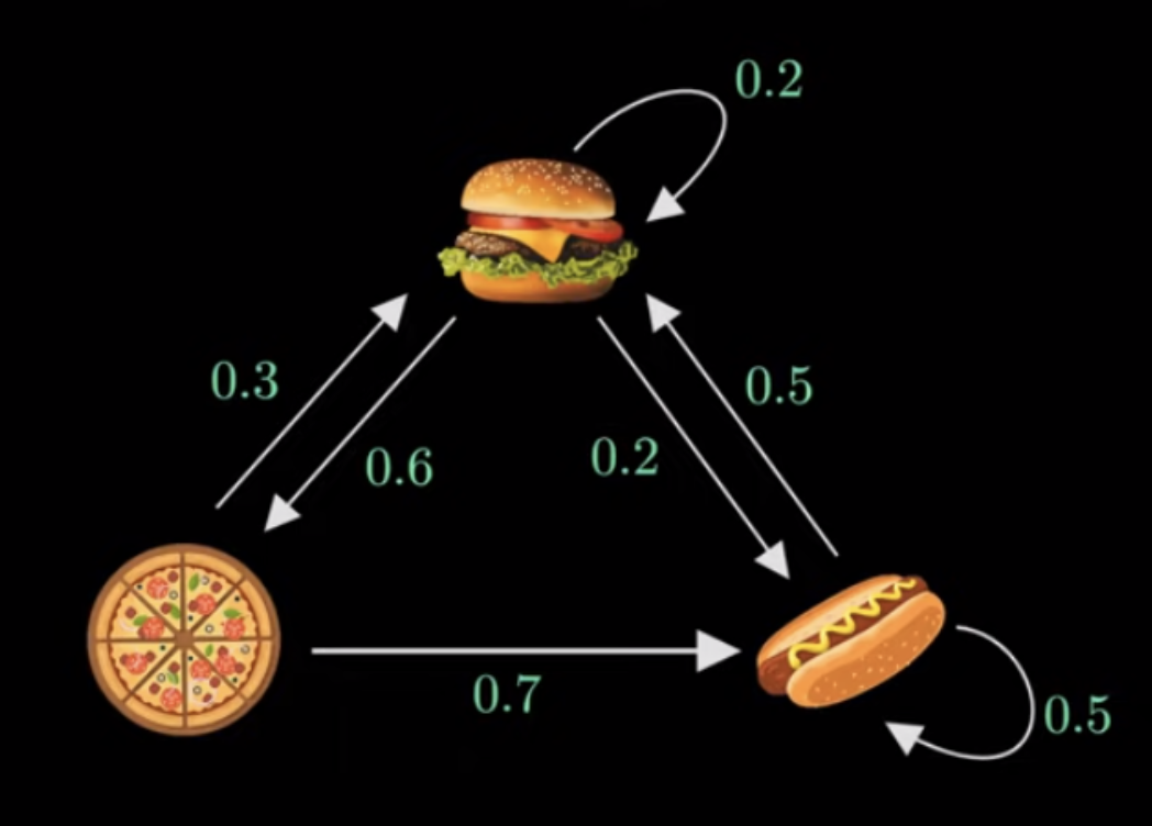
Taking state 1 to be hamburger, state 2 to be pizza and state 3 to be hotdog, the transition matrix \(P\) can be written as \[ P=\begin{bmatrix} 0.2 & 0.6 & 0.2 \\ 0.3 & 0 & 0.7 \\ 0.5 & 0 & 0.5 \end{bmatrix}. \]
Given the restaurant first serves pizza we can define the initial distribution \(\pi_{0}=\begin{bmatrix}0 & 1 & 0\end{bmatrix}\). Applying the transition matrix \(P\) we get \[ \pi_{0}P=\begin{bmatrix} 0 & 1 & 0 \end{bmatrix}\cdot \begin{bmatrix} 0.2 & 0.6 & 0.2 \\ 0.3 & 0 & 0.7 \\ 0.5 & 0 & 0.5 \end{bmatrix}=\begin{bmatrix} 0.3 & 0 & 0.7 \end{bmatrix}=\pi_{1}, \]
the second state future transition probabilities. Repeating this step for \(\pi_{1}\) we have \[ \pi_{0}P=\begin{bmatrix} 0.3 & 0 & 0.7 \end{bmatrix}\cdot \begin{bmatrix} 0.2 & 0.6 & 0.2 \\ 0.3 & 0 & 0.7 \\ 0.5 & 0 & 0.5 \end{bmatrix}=\begin{bmatrix} 0.41 & 0.18 & 0.41 \end{bmatrix}=\pi_{2}, \]
If a stationary distribution \(\pi\) exists it would mean that as \(\pi_{0}, \pi_{1}, \dots\) continues, eventually it will reach a point where it doesn’t change when \(P\) is applied, hence using linear algebra we can write the expression \[ \pi P=\pi, \]
see Definition 2 above. Additionally, since \(\pi\) is a vector of probabilities we have that \(\pi(1)+\pi(2)+\pi(3)=1\) and solving this system gives the stationary distribution \[ \pi=\begin{bmatrix} \frac{25}{71} & \frac{15}{71} & \frac{31}{71} \end{bmatrix}. \]
We can numerically confirm our result by iteratively applying the transition probability matrix:
P = np.array([
    [.2, .6, .2],
    [.3, 0, .7],
    [.5, 0, .5]
])
pi = np.array([
    0, 1, 0
])
pi_list = []
pi_list.append(pi)

n = 50

for _ in range(n):
    pi = pi @ P
    pi_list.append(pi)

pi_list = np.array(pi_list).squeeze()
fig, ax = plt.subplots()
ax.plot(range(n+1), pi_list[:,0], color="red", label="Hamburger")
ax.plot(range(n+1), pi_list[:,1], color="green", label="Pizza")
ax.plot(range(n+1), pi_list[:,2], color="blue", label="Hotdog")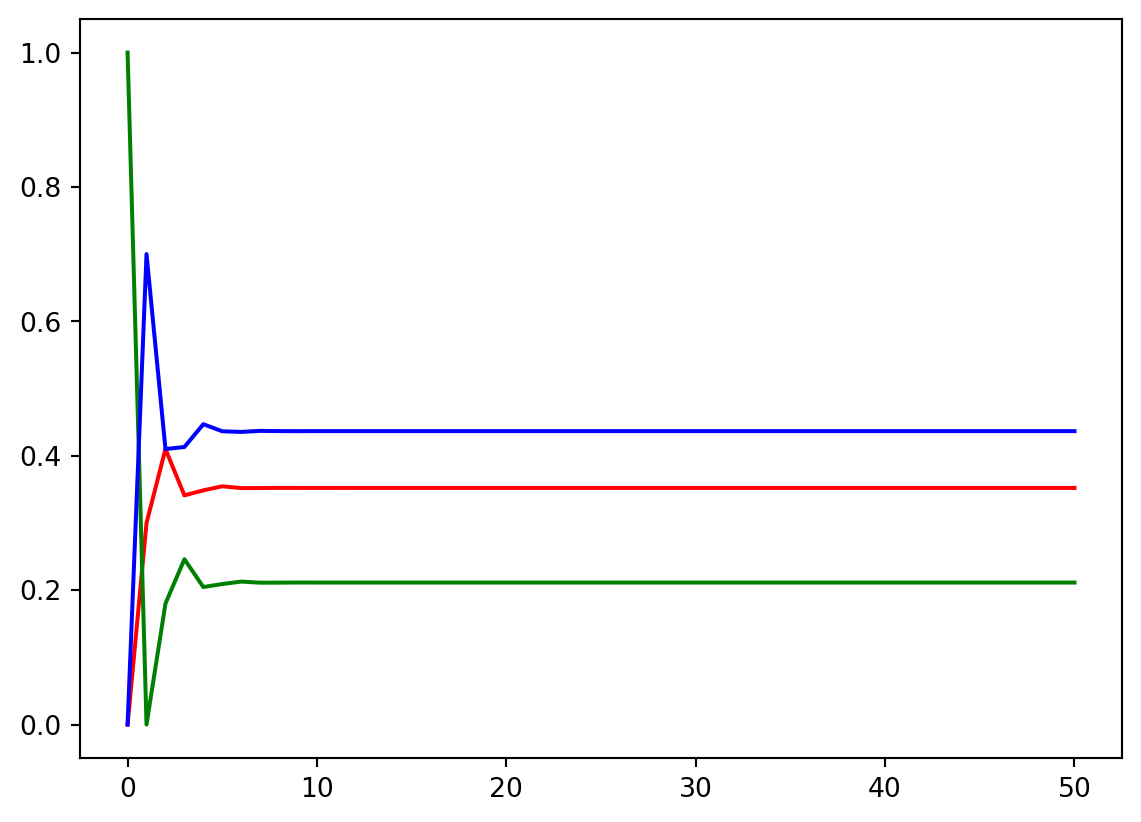
Definition: (Doubly Stochastic Matrices)
A matrix \(P:=(p_{i,j})_{i,j\in\mathcal{S}}\) is said to be doubly stochastic when both rows and columns sum to 1, that is \[
\sum_{j\in\mathcal{X}}p_{i,j} = \sum_{i\in\mathcal{X}}p_{i,j}=1.
\]
Theorem: (Uniform Stationary Distributions for Doubly Stochastic MCs)
A finite state homogenous MC with doubly stochastic transition probability matrix has a uniform stationary distribution.
Proof
Assume \(\mathcal{X}\) has \(n\) elements and define \(\pi = (\pi_i)_{i\in\mathcal{X}}\) where \(\pi_i=1/n\). Then clearly
\[ \sum_{i\in\mathcal{X}} \pi_i p_{i,j} = \frac{1}{n}\sum_{i\in\mathcal{X}}p_{i,j} = \frac{1}{n} = \pi_j, \]
holds for all \(j\in\mathcal{X}\). Since by definition \(\pi\) is normalized we obtain the result.
\(\square\)