Probability Theory & Statistics - Probability Distributions
A summary of all standard probability distributions.
1 Probability Distributions & Random Variables
1.1 Random Variables
A random variable is a numerical description of the outcome of a statistical experiment. A random variable that may assume only a finite number or an infinite sequence of values is said to be discrete; one that may assume any value in some interval on the real number line is said to be continuous.
1.2 Probability Distributions of Random Variables
A probability distribution is a mathematical function that gives the probability of occurrence of different possible outcomes for an experiment. It is therefore a mathematical description of a random phenomenon in terms of its sample space and the probabilities of events (subsets of a sample space).
Generally, a probability distribution can be described by a probability function $P:\mathcal{A}\rightarrow\R$ where $\mathcal{A}$ is the input space which is related to the sample space of the experiment and gives a real number probability as an output.
The above probability function only characterizes a probability distribution if it satisfies all the Kolmogorov axioms, which are defined by:
- Probability is non-negative: $P(X\in E)\geq 0, \forall E\in \mathcal{A}$;
- No probability exceeds 1: $P(X\in E)\leq 1, \forall E \in\mathcal{A}$;
- The probability of $P(X\in\bigcup_i E_i)=\sum_i P(X\in E_i).$
The concept of a probability function is made more rigorous in measure theory which we will discuss further in a separate article.
Discrete Probability Distributions
The probability distribution for a random variable describes how the probabilities are distributed over the values of the random variable. For a discrete random variable, $x$, the probability distribution is defined by a probability mass function, denoted by $f(x)$. This function provides the probability for each value of the random variable.
In the development of the probability function for a discrete random variable, two conditions must be satisfied:
-
$f(x)$ must be non-negative for each value of the random variable, and
-
The sum of the probabilities for each value of the random variable must equal one.
Continuous Probability Distributions
A continuous random variable may assume any value in an interval on the real number line or in a collection of intervals. Since there is an infinite number of values in any interval, it is not meaningful to talk about the probability that the random variable will take on a specific value; instead, the probability that a continuous random variable will lie within a given interval is considered.
In the continuous case, the counterpart of the probability mass function is the probability density function, also denoted by $f(x)$. For a continuous random variable, the probability density function provides the height or value of the function at any particular value of $x$; it does not directly give the probability of the random variable taking on a specific value. However, the area under the graph of $f(x)$ corresponding to some interval, obtained by computing the integral of $f(x)$ over that interval, provides the probability that the variable will take on a value within that interval.
A probability density function must satisfy two requirements:
-
$f(x)$ must be non-negative for each value of the random variable, and
-
The integral over all values of the random variable must equal one.
2 Basic Terms
We are usually interested in describing the shape and properties of a distribution that we are considering. We therefore introduce and describe the following basic terms:
-
Mode
For a discrete random variable, the mode is the value with the highest probability. For a continuous random variable, the mode is the location at which the pdf has a local peak.
-
Support
The support of a distribution is the set of values that can be assumed with non-zero probability by the random variable.
-
Tail
The tails of a distribution are the regions close to the bounds of the random variable.
-
Head
The head of a distribution is the region where the distribution is relatively high,
-
Mean
The mean (expected value) of a distribution is the weighted average of the possible values, using their probabilities as weights.
-
Median
The median of a distribution is the value such that the set of values less than the median, and the set greater than the median, each have probabilities no greater than 0.5.
-
Variance
The variance of a distribution is the second moment of the pmf or pdf about the mean. It is an important measure of the dispersion of a distribution.
-
Standard Deviation
The standard deviation of a distribution is the square root of the variance. It is another important measure of the dispersion of a distribution.
-
Quantile
The q-quantile of a distribution is the value $x$ such that $P(X<x)=q$.
-
Symmetry
A distribution is symetric if their exists a line of symmetry in the distribtion plot.
-
Skewness
The skewness of a distribution measures the extent to which a distribution “leans” to one side of its mean. It is the third standardised moment of the distribution.
-
Kurtosis
The kurtosis of a distribution is a measure of the “fatness” of the tails of a distribution. It is the fourth standardised moment of the distribution.
-
Continuity
A distribution exhibits continuity if its values do not change abruptly.
3 Basic Distributions
There is a large number of different distributions which are suitable in a variety of situations. The most common of these distributions are:
-
The uniform distribution;
-
The Bernoulli distribution;
-
The binomial (& negative binomial) distribution;
-
The geometric (& hypergeometric) distribution;
-
The Poisson distribution;
-
The exponential distribution;
-
The Weibull distribution;
-
The normal (Gaussian) distribution;
-
The log-normal distribution;
-
The student-t distribution;
-
The chi-squared distribution;
-
The gamma distribution;
-
The beta distribution.
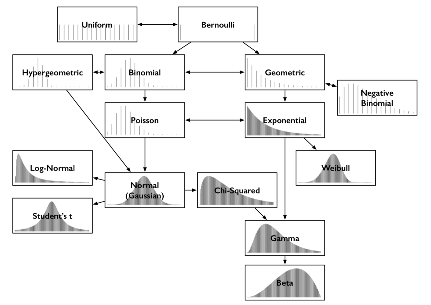
These common distributions relate to each other in intuitive and interesting ways. These relationships are highlighted in Figure 1.

3.1 The Uniform Distribution
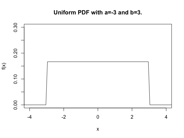
The uniform distribution describes any situtation in which every outcome in a sample space is equally likely. It has both a discrete form - e.g. rolling a single standard die - and a continuous form. A uniform probability distribution describes an experiment where there is an arbitrary outcome that lies between bounds which are defined by the finite parameters $a$ and $b$.
Uniform Probability Density Function
The probability density function of the continuous uniform distribution is given by:
\[f(x)=\begin{cases}\frac{1}{b-a}\quad\text{for}\quad a\leq x\leq b,\\ 0\quad\text{otherwise.}\end{cases}\]
We produce a plot of the uniform distribution function for the bounds $a=-3$ and $b=3$, shown below in Figure 2.
Uniform Cumulative Distribution Function
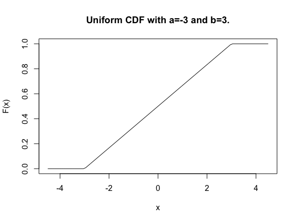
The uniform cumulative distribution function is given by:
\[F(x)=\begin{cases}0\quad\text{for}\quad x<a\\\frac{x-a}{b-a}\quad\text{for}\quad a\leq x \leq b\\1\quad\text{for}\quad x>b.\end{cases}\]
We produce a plot of the uniform cumulative distribution function for the example above, shown below in Figure 3.
Uniform Summary Statistics
| Statistic | Formula |
|---|---|
| Mean | $\frac{1}{2}(a+b)$ |
| Variance | $\frac{1}{12}(b-a)^2$ |
| Skewness | $0$ |
| Kurtosis | $-\frac{6}{5}$ |
3.2 The Bernoulli Distribution
The Bernoulli distribution is the discrete probability distribution of a random variable which takes the value of 1 with probabiity $p$ and the value 0 with probability $1-p$. It can be thought of as a model for the set of possible outcomes of any single experiment that asks a yes or no question.
Bernoulli Probability Mass Function
The Bernoulli probability mass function is given by:
\[f(k) = \begin{cases}p\quad\text{for}\quad k=1;\\ q=1-p\quad\text{for}\quad k=0.\end{cases}\]
Bernoulli Cumulative Distribution Function
The Bernoulli cumulative distribution function is given by:
\[F(k)=\begin{cases}0\quad \text{for}\quad k<0\\ 1-p\quad\text{for}\quad 0\leq k < 1\\ 1\quad\text{for}\quad k\geq 1.\end{cases}\]
Bernoulli Summary Statistics
| Statistic | Formula |
|---|---|
| Mean | $p$ |
| Variance | $pq$ |
| Skewness | $\frac{qp}{\sqrt{pq}}$ |
| Kurtosis | $\frac{1-6pq}{pq}$ |
3.3 The Binomial Distribution
The binomial distribution with parameters $n$ and $p$ is the discrete probability distribution of the number of successes in a sequence of $n$ independent Bernoulli trials.
Binomial Probability Mass Function
For a random variable following a binomial distribution $X\sim\text{Binomial}(n, p)$ the probability mass function is given by:
\[f(k) = {n\choose k} p^k(1-p)^{n-k};\]
for $k=0,1,…,n$, and where ${n\choose k}=\frac{n!}{k!(n-k)!}$.
Binomial Cumulative Distribution Function
The binomial cumulative distribution function is given by:
\[F(k)=\sum_{i=0}^{\lfloor k\rfloor}{n\choose i}p^i(1-p)^{n-i};\]
where $\lfloor k\rfloor$ is the floor under $k$, i.e. the greatest integer less than or equal to $k$.
Binomial Summary Statistics
| Statistic | Formula |
|---|---|
| Mean | $np$ |
| Variance | $npq$ |
| Skewness | $\frac{q-p}{\sqrt{npq}}$ |
| Kurtosis | $\frac{1-6pq}{npq}$ |
3.4 The Geometric Distribution
The geometric distribution is the discrete probability distribution of the number of failures before the first success, supported on the set ${0,1,2,…}$.
Geometric Probability Mass Function
For a random variable following a geometric distribution $X\sim\text{Geometric}(p)$ the probability mass function is given by:
\[f(k) = (1-p)^{k}p,\]
for $k\in\Z^+$.
Geometric Cumulative Distribution Function
The geometric cumulative distribution function is given by:
\[F(k)=1-(1-p)^{k+1}.\]
Geometric Summary Statistics
| Statistic | Formula |
|---|---|
| Mean | $\frac{1-p}{p}$ |
| Variance | $\frac{1-p}{p^2}$ |
| Skewness | $\frac{2-p}{\sqrt{1-p}}$ |
| Kurtosis | $6+\frac{p^2}{1-p}$ |
3.5 The Poisson Distribution
The Poisson distribution is a discrete probability distribution that describes the porbability of a given number of events occuring in a fixed interval of time (or space) if these events occur with a known comstant mean rate and independently of the time since the last event.
Poisson Probability Mass Function
For a random variable following a Poisson distribution $X\sim \text{Poisson}(\lambda)$, the probability mass function is given by:
\[f(k)=\frac{\lambda^k e^{-\lambda}}{k!},\]
where $k$ is the number of occurrences.
Poisson Cumulative Frequency Distribution
The Poisson cumulative frequency distribution is given by:
\[e^{-\lambda}\sum_{i=0}^{\lfloor k \rfloor}\frac{\lambda^i}{i!}.\]
Poisson Summary Statistics
| Statistic | Formula |
|---|---|
| Mean | $\lambda$ |
| Variance | $\lambda$ |
| Skewness | $\lambda^{-\frac 12}$ |
| Kurtosis | $\lambda^{-1}$ |
3.6 The Exponential Distribution
The exponential distribution is the continuous distribution describing tje time between events in a Poisson point process. It is a particular case of the gamma distribution - see below.
Exponential Probability Density Function
For a random variable following an exponenital distribution $X\sim\text{Exponential}(\lambda)$, the probability distribution function is given by:
\[f(x)=\begin{cases}\lambda e^{\lambda x}\quad\text{for}\quad x\geq 0,\\0\quad\text{for}\quad x<0,\end{cases}\]
where $\lambda>0$ is the rate parameter.
Exponential Cumulative Frequency Distribution
The exponential cumulative frequency distribution is given by:
\[F(x)=\begin{cases}1-e^{-\lambda x}\quad\text{for}\quad x\geq 0,\\ 0\quad\text{otherwise}.\end{cases}\]
Exponential Summary Statistics
| Statistic | Formula |
|---|---|
| Mean | $\frac{1}{\lambda}$ |
| Variance | $\frac{1}{\lambda^2}$ |
| Skewness | $2$ |
| Kurtosis | $6$ |
3.7 The Weibull Distribution
The Weibull distribution is a continuous probability distribution which is used extensively in reliability applications to model failure times.
Weibull Probability Distribution Function
For a random variable following a Weibull distribution $X\sim\text{Weibull}(\lambda, k)$, the probability distribution function is given by:
\[f(x)=\begin{cases}\frac k\lambda\left(\frac x\lambda\right)^{k-1}e^{\left(x/ \lambda\right)^k}\quad\text{for}\quad x\geq 0\\ 0\quad\text{otherwise},\end{cases}\]
where $k>0$ is the shape parameter and $\lambda>0$ is the scale parameter.
Weibull Cumulative Distribution Function
The Weibull cumulative distribution function is given by:
\[F(x)=\begin{cases}1-e^{-(x\lambda)^k}\quad\text{for}\quad x\geq 0,\\0\quad\text{otherwise}.\end{cases}\]
Weibull Summary Statistics
| Statistic | Formula |
|---|---|
| Mean | $\lambda \Gamma (1 + 1/k)$ |
The gamma function $\Gamma(x)$ is defined by:
\[\Gamma(x)=(n-1)!,\]
for any positive integer $n$.
We only list the mean due to the length of the definitions of the other summary statistics.
3.8 The Normal (Gaussian) Distribution
The normal (or Gaussian) distribution is a continuous probability distribution for a real-valued random variable. Normal distributions are important in statistics, partly due to the central limit theorem which states that under certain conditions, the average of many samples (observations) of a random variable with finite mean and variance is itself a random variable—whose distribution converges to a normal distribution as the number of samples increases.
Normal Probability Distribution Function
For a random variable following a normal distribution $X\sim\text{Normal}(\mu, \sigma)$, the proability distribution function is given by:
\[f(x) = \frac{1}{\sigma\sqrt{2\pi}}\exp\left(-\frac{1}{2}\left(\frac{x-\mu}{\sigma}\right)^2\right),\]
where $\mu$ is the mean of the distribution and $\sigma$ is its standard deviation.
The normal distribution is sometimes informally called a bell curve due to the shape of its distribution plot. We generate 10,000 realisations of a normal random variable with $\mu=0$ and $\sigma=1$. We then produce a histogram of these data points which displays the empirical distribution of the dataset before plotting an overlying plot of the corresponding normal distribution plot. This is shown below in Figure 3.
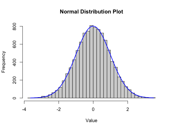
We calculate the empirical mean and standard deviation of the data to be $\mu=-0.007187947$ and $\sigma=0.9950355$, extremely close to the underlying distribution values.
3.8 The Log-Normal Distribution
The log-normal distribution is a *continuous probability distribution of a random variable whose logarithm is normally distributed.
Log-Normal Probability Distribution
For a random variable following a log-normal distribution $X\sim\text{Log-Normal}(\mu, \sigma)$, the probability distribution function is given by:
\[f(x)=\frac{1}{x\sigma\sqrt{2\pi}}\exp\left(-\frac{(\ln(x)-\mu)^2}{2\sigma^2}\right).\]
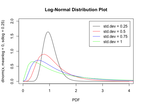
We demonstrate the various shapes of the log-normal distribution below in Figure 4.
3.9 The Student-t Distribution
The student-t distribution is any member of a family of continuous probability distributions that arise when estimating the mean of a normally distributed populations in situations where the sample size is small and the population’s standard deviation is unknown.
The t-distribution is symmetric and bell-shaped - like the normal distribution - but with heavier tails meaning that it is more prone to producing values that fall far from its mean.
Student-t Probability Distribution Function
For a random variable following a student-t distribution $X\sim\text{Student-t}(\upsilon)$, the probability distribution function is given by:
\[f(x)=\frac{\Gamma\left(\frac{\upsilon +1}{2}\right)}{\sqrt{\upsilon\pi}\Gamma\left(\frac{\upsilon}{2}\right)}\left(1+\frac{t^2}{\upsilon}\right)^{-\frac{\upsilon +1}{2}},\]
where $\upsilon$ is the number of degrees of freedom.
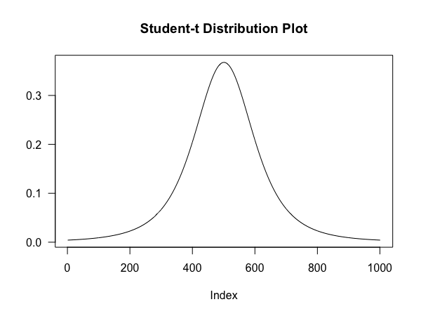
We produce a plot of the student-t distribution function with $\upsilon=3$, shown below in Figure 5.
3.10 The Chi-Squared Distribution
The chi-squared distribution is the continuous distribution describing the sum of the squares of $k$ independent standard normal random variables. It is the special case of the gamma distribution and is one of the most widely used probability distribution in inferential statistics, notably in hypothesis testing and in construction of confidence intervals.
Chi-Squared Probability Density Function
For a random variable following a chi-squared distribution $X\sim\Chi^2(k)$, the probability distribution function is given by:
\[f(x)=\frac{1}{2^{k/2}\Gamma(k/2)}x^{(k/2)-2}\exp\left(-\frac x 2\right),\]
where $k\in\N^*$ is the degrees of freedom.
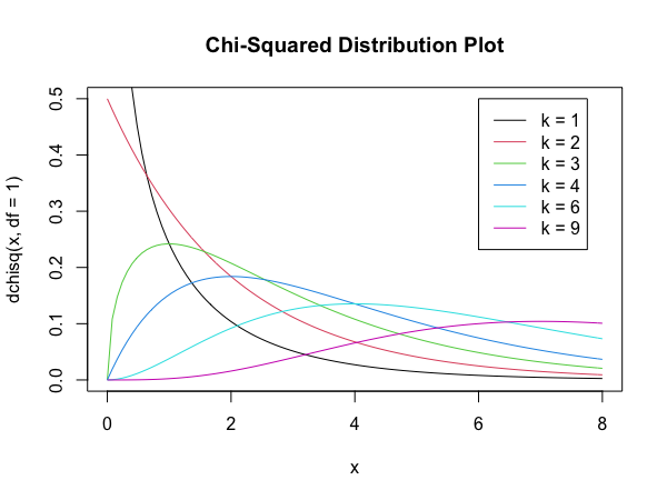
We produce a plot of the student-t distribution function with various degrees of freedom, shown below in Figure 6.
3.11 The Gamma Distribution
The gamma distribution is a two-parameter family of continuous probability distributions. The gamma distribution requires a shape parameter $k$ and a scale parameter $\theta$.
Gamma Probability Distribution Function
For a random variable following a gamma probability distribution $X\sim\text{Gamma}(k, \theta)$, the probability distribution function is given by:
\[f(x)=\frac{1}{\Gamma(k)\theta^k}x^{k-1}\exp\left(-\frac{x}{\theta}\right),\]
where $k$ is the shape parameter and $\theta$ is the scale parameter.
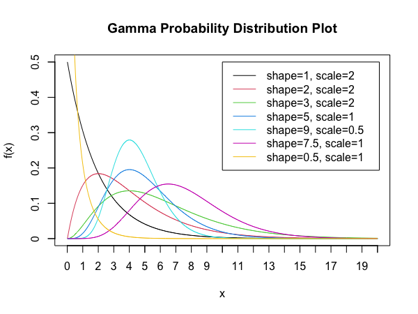
We produce a plot of the gamma distribution function with various shape and scale parameters, shown below in Figure 7.
3.12 The Beta Distribution
The beta distribution is a family of continuous probability distributions defined on the interval $[0,1]$ parameterised by two positive shape parameters denoted by $alpha$ and $beta$. The beta distribution has been applied to model the behaviour of random variables limited to intervals of finite length in a wide variety of disciplines.
Beta Probability Distribution Function
For a random variable $X\sim\text{Beta}(\alpha, \beta)$, the probability distribution function is given by:
\[\frac{\Gamma(\alpha + \beta)}{\Gamma(\alpha)\Gamma(\beta)}x^{\alpha-1}(1-x)^{\beta-1},\]
where $\alpha, \beta>0$ are the shape parameters.
We include an animated plot of the various shapes of the Beta distribution - created by Pabloparsil.

4 Probability Distributions in Finance
Probability distributions are used very frequently in finance to model financial data such as stock returns. Stock returns are often assumed to follow a normal distribution, however they typically exhibit large negative and positive returns which occur more than expected if they followed a normal distribution. Furthermore, since stock prices are bounded by zero but have a potentially unlimited upside, the distribution of stock returns is often considered to be log-normal - evidence of which is provided by the thick tails of their distribution.
Probability distributions are often also used in risk management and to evaluate the probability and amount of losses that an investment portfolio would incur based on a distribution of historical returns. A popular risk measure used in investing is Value-at-Risk (VaR) which yields the minimum loss that can occur given a probability and time frame for a portfolio.
References
-
Common Probability Distributions: The Data Scientist’s Crib Sheet, medium.com, Sean Owen, June 29, 2018.
-
Probability Distribution, investopedia.com, Adam Hayes, October 29, 2020.
-
Probability distribution, wikipedia.com.
